In this Topic Hide
There are many types of fixed probe as described in the following table
| Probe Type | Description | To Place |
|---|---|---|
| Voltage | Single ended voltage. Hint: If you place the probe immediately on an existing schematic wire, it will automatically be given a meaningful name related to what it is connected to |
Menu:
Hot key: B |
| Current | Device pin current. A single terminal device to place over a device pin |
Menu:
Hot key: U |
| Inline current | In line current. This is a two terminal device that probes the current flowing through it. | Menu: |
| Differential voltage | Probe voltage between two points | Menu: |
| dB | Probes db value of signal voltage. Only useful in AC analysis | Menu: |
| Phase | Probes phase of signal voltage. Only useful in AC analysis | Menu: |
| Bode plot with Measurements | Plots db and phase of vout/vin. Connect to the input and output of a circuit to plot its gain and phase. Includes optionsl measurements for phas margin, gain margin and gain crossover frequency | Menu: |
| Bode plot - basic version | Plots db and phase of vout/vin. Connect to the input and output of a circuit to plot its gain and phase. | Menu: |
| Bus plot | Plots bus signal in 'logic analyser' style | Menu: |
| Power plot | Plots the power in a device. The power probe must be attached to a single pin of the device. It doesn't matter which pin - the power plotted in the instantaneous power in the whole device | Menu: |
| Per Cycle | Plot a graph based on a calculation performed for each complete cycle of a repetitive waveform. See Per Cycle Probes | Available from Parts Selector |
| X-Y | Plot a graph of one signal on the y-axis with respect to a second signal on the x-axis. See X-Y Probes | Menu: |
Current probes and power probes must be placed directly over a part pin. They will have no function if they are not and a warning message will be displayed.
All probe types have a large number of options allowing you to customise how you want the graph plotted. For many applications the default settings are satisfactory. In this section, the full details of available probe options are described. Select the probe and press F7 or menu Edit Part...
The following dialog will be displayed for voltage, current, power, db and phase probes:
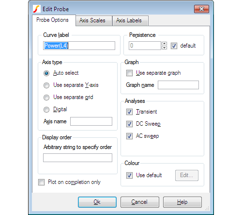
The elements of each tabbed sheet are explained below.
| Curve Label | Text displayed by the probe on the schematic and also used to label the resulting curves | ||||||||
| Persistence |
The number of curves from a single probe that will be displayed at once.
To set the persistence value in general options, follow these steps:
|
||||||||
|
Axis type |
Specifies the type of y-axis to use for the curve.
|
||||||||
|
Graph |
Check Use Separate Graph to create a new graph sheet for the probe. You may also supply a graph name, which works the same way as axis name described above. this is not a label but a means of identification. Any other probes using the same graph name will have their curves directed to the same graph sheet. | ||||||||
|
Analyses |
Specifies for which analyses the probe is enabled. Note: Other analysis modes such as noise and sensitivity are not included because these do not support schematic cross probing of current or voltage. For SIMPLIS mode, a Periodic Operating Point (POP) option is also available. |
||||||||
|
Display order |
Enter a string to control the grid display order. The value is arbitrary and will not be displayed. To force the curve to be placed above other curves that don't use this value, prefix the name with '!'. The '!' character has a low ASCII value. Conversely, use '~' to force curve to be displayed after other curves. |
||||||||
|
Colour |
Check Use default to minimise duplicate colours on the same graph by allowing the colour to be chosen automatically. Alternatively uncheck, this box and then press Edit... to select a colour of your choice. In this case the trace always has the same colour. | ||||||||
|
Plot on completion only |
|
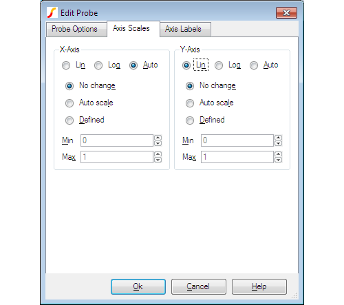
| Parameter | Description |
| Lin/Log/Auto |
Specify whether you want X-Axis to be linear or logarithmic.
|
|
No Change Auto scale Defined |
Controls how the axis limits are defined
|
This sheet has four edit boxes allowing you to specify, x and y axis labels as well as their units. If any box is left blank, a default value will be used or will remain unchanged if the axis already has a defined label.
Select device and press F7 in the usual manner. A dialog box will show similar to that shown in Bus Probe Options. But you will notice an additional tabbed sheet titled Probe Options. This allows you to select an axis type and graph in a similar manner to that described above for fixed voltage and current probes.
Fixed probes may successfully be used in hierarchical designs. If placed in a child schematic, a plot will be produced for all instances of that child and the labels for each curve will be prefixed with the child reference.
When you add a fixed single ended voltage or current probe after a run has started, the graph of the probed point opens soon after resuming the simulation. To do this:
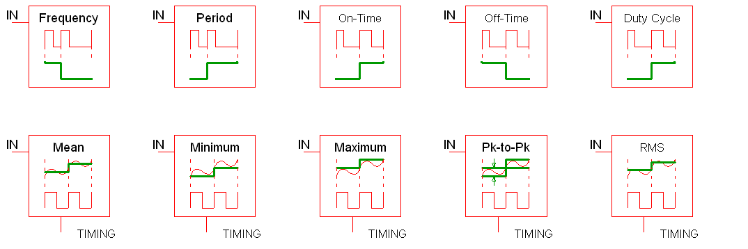
Per Cycle Probes first calculate a new curve based on a built-in formula and then plot the curve on a graph. The input can be one of the following:
The Per-cycle Probe specification is shown in the following table:
| Per-cycle Probes | |
|---|---|
| Model Name: | Per Cycle Probes |
| Simulator: | The device is compatible with the SIMetrix and SIMPLIS simulators |
| SIMetrix Parts Selector Location: |
|
| SIMPLIS Parts Selector Location: |
|
|
Symbol Library: |
None the symbol is automatically generated when placed |
| Symbols: |
|
| Multiple Selections: |
Multiple probes can be selected and edited simultaneously.
|
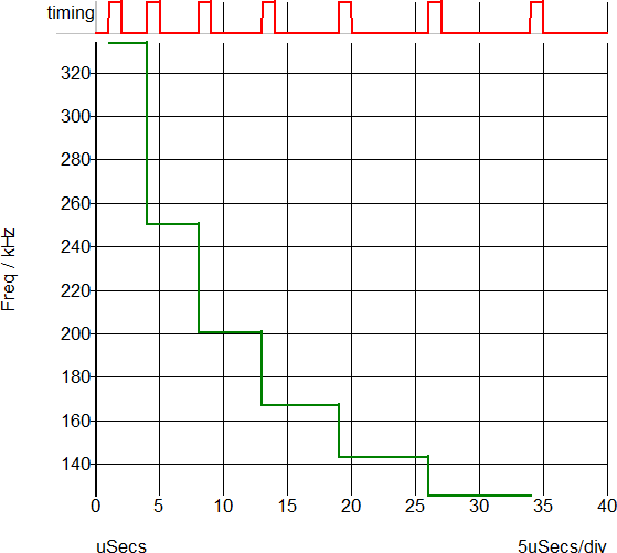
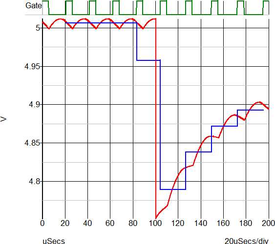
These advanced probes allow you to visualize subtle behaviour which is not otherwise easy to see. One example is to visualize how the switching frequency varies over the simulation time window. In this case, the probe first finds all edges which match the trigger conditions and then calculates a new curve with the frequency measurements on the vertical axis and the input time vector on the horizontal axis. An example waveform showing a pulse train and the per cycle frequency of the curve is shown below:
The per-cycle measurement can also be applied to amplitude of an input voltage or current. For example, you can plot the mean value of a switching power converter output with the mean value being calculated on a per-cycle basis. This example is show below - the mean value of a converter output voltage is plotted in a per-cycle manner. The gate voltage is used to determine the timing edge information.
To configure the Per Cycle Probe, follow these steps:
The following tab allows you to define general probe options, which are explained in the table below.

| Parameter | Description | ||||||||
| Measurement | Frequency, Period, On-Time, Off-Time, Duty Cycle, Mean Maximum, Minimum, Peak-to-Peak, or RMS | ||||||||
|
Edge Direction |
Rising, Falling or Both | ||||||||
| Curve type | Stepped or Smooth | ||||||||
| Curve Label | Text displayed by the probe on the schematic and also used to label the resulting curves | ||||||||
| Persistence |
The number of curves from a single probe that will be displayed at once.
To set the persistence value in general options, follow these steps:
|
||||||||
|
Axis type |
Specifies the type of y-axis to use for the curve.
|
||||||||
|
Graph |
Check Use Separate Graph to create a new graph sheet for the probe. You may also supply a graph name, which works the same way as axis name described above. this is not a label but a means of identification. Any other probes using the same graph name will have their curves directed to the same graph sheet. | ||||||||
|
Analyses |
Specifies for which analyses the probe is enabled. Note: Other analysis modes such as noise and sensitivity are not included because these do not support schematic cross probing of current or voltage. For SIMPLIS mode, a Periodic Operating Point (POP) option is also available. |
||||||||
|
Display order |
Enter a string to control the grid display order. The value is arbitrary and will not be displayed. To force the curve to be placed above other curves that don’t use this value, prefix the name with '!'. The '!' character has a low ASCII value. Conversely, use '~' to force curve to be displayed after other curves. |
||||||||
|
Colour |
Check Use default to minimise duplicate colours on the same graph by allowing the colour to be chosen automatically. Alternatively uncheck, this box and then press Edit... to select a colour of your choice. In this case the trace always has the same colour. | ||||||||
|
Plot on completion only |
This option is not available with per-cycle probes and the setting of the check box will be ignored.
|
The following tab allows you to define the scale for the X-axis and for the Y-axis as explained in the table below.
| Parameter | Description |
| Lin/Log/Auto |
Specify whether you want X-Axis to be linear or logarithmic.
|
|
No Change Auto scale Defined |
Controls how the axis limits are defined
|
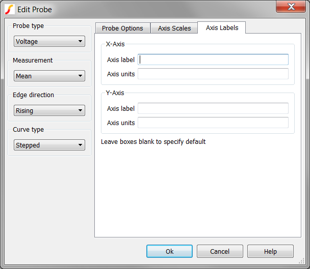
To specify axis labels and units, click the Axis Labels tab, and enter values as needed.
Note: If any box is left blank, a default value is used or remains unchanged if the axis already has a defined label.
XY Probes plot two curves against each other in an XY plot. Each input can be either differential voltage or inline current, and the curves can be output to any graph and axis. XY probes are available in both SIMetrix and SIMPLIS. The XY Probe specification is shown in the following table:
| XY Probes | |
|---|---|
| Model Name: | XY Probe |
| Simulator: | This device is compatible with the SIMetrix and SIMPLIS simulators. |
| Part Selector Location: | |
| Symbol Library: | connection.sxslb |
| Symbols: |

|
| Multiple Selections: | Multiple probes can be selected and edited simultaneously. |
|
|
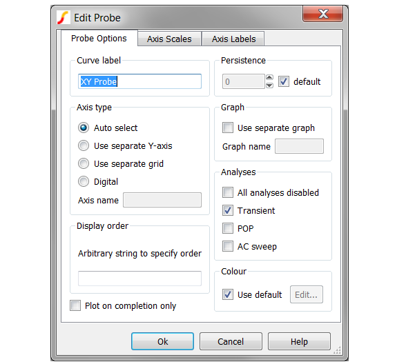
To configure the XY Probe, follow these steps:
The following tab allows you to define general probe options, which are explained in the table below.
| Curve Label | Text displayed by the probe on the schematic and also used to label the resulting curves | ||||||||
| Persistence |
The number of curves from a single probe that will be displayed at once.
To set the persistence value in general options, follow these steps:
|
||||||||
|
Axis type |
Specifies the type of y-axis to use for the curve.
|
||||||||
|
Graph |
Check Use Separate Graph to create a new graph sheet for the probe. You may also supply a graph name, which works the same way as axis name described above. this is not a label but a means of identification. Any other probes using the same graph name will have their curves directed to the same graph sheet. | ||||||||
|
Analyses |
Specifies for which analyses the probe is enabled. Note: Other analysis modes such as noise and sensitivity are not included because these do not support schematic cross probing of current or voltage. For SIMPLIS mode, a Periodic Operating Point (POP) option is also available. |
||||||||
|
Display order |
Enter a string to control the grid display order. The value is arbitrary and will not be displayed. To force the curve to be placed above other curves that don’t use this value, prefix the name with '!'. The '!' character has a low ASCII value. Conversely, use '~' to force curve to be displayed after other curves. |
||||||||
|
Colour |
Check Use default to minimise duplicate colours on the same graph by allowing the colour to be chosen automatically. Alternatively uncheck, this box and then press Edit... to select a colour of your choice. In this case the trace always has the same colour. | ||||||||
|
Plot on completion only |
This option is not available with XY Probes and the check box setting will be ignored.
|
| Parameter | Description |
| Lin/Log/Auto |
Specify whether you want X-Axis to be linear or logarithmic.
|
|
No Change Auto scale Defined |
Controls how the axis limits are defined
|
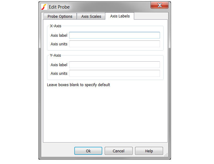
To specify axis labels and units, click the Axis Labels tab, and enter values as needed.
Note: If any box is left blank, a default value is used or remains unchanged if the axis already has a defined label.
The Bode Plot Probe with Measurements generates plots for the gain and phase of the ratio of two voltages. The probe can be configured to plot only the gain or phase, or both gain and phase.
| Summary - Bode Plot Probe with Measurements | |
|---|---|
| Model Name | Bode Plot Probe |
| Simulator | This device is compatible with both SIMetrix and SIMPLIS simulators |
| Schematic Menu | |
| Parts Selector | |
| Symbol Library | Connections |
| Model File | none |
| Symbol |

|
| Multiple Selections | If multiple Bode plot probes are selected before editing, all properties except the curve labels can be simultaneously changed for all probes. The curve label properties will remain unchanged for all selected probes |
| Usage | This schematic probe symbol plots the magnitude and phase of the ratio of two complex voltages, OUT/IN. The magnitude can be plotted in db or volts/volts; the horizontal axis scale is determined by the simulation sweep type. If the simulation is swept in log frequency steps, the horizontal axis will automatically be log scaled |
To configure the Bode Plot Probe with Measurements, follow these steps:

| Options - Bode Plot Probe with Measurements | |
|---|---|
| Use separate graph | Check this option in order to supply an alias for each output graph tab |
| Graph name | The Graph name is an alias for each output graph tab and will not be visible on the graph output. Curves with the same graph name property will be output on the same graph tab. Graph name be safely ignored unless multiple Bode plot probes are used. Use separate graph must be checked to supply this name. |
| Disable gain/phase | Check this box to disable both gain and phase graphs |
| Persistence |
The Persistence property determines when previous simulation data is deleted from the graph viewer. If Use default is checked or if the persistence is set to -1, the probe uses the default global persistence value.
The default persistence can be set from the command shell menu:
|
| Curve label | Sets the name of the curve. Note: This field appears in both the Gain and Phase groups on the dialog |
| Y axis label | Sets the Y axis label for the individual gain and phase axes. When multiple curves from multiple probes are placed on the same axis, the axis label properties must be identical or the axis label is blank. If this field is left blank, the axis label appears with the name specified in the Curve label field. Note: This field appears in both the Gain and Phase groups on the dialog |
| Vertical scale |
Allows you to select the function to perform on the simulation data.
|
| Curve |
Selects the Phase curve offset
|
| Vertical axis |
This group has two options:
Vertical limits
|
| Colour |
Defines colours for the curves:
The change the default sequence of colours from the command shell menu, select For additional information see Colours and Fonts. Note: This field appears in both the Gain and Phase groups on the dialog. |
| Display curves on | Allows you to define the number of grids in the output: Single grid or Two grids |
| Vertical order |
Allows you to specify the order of the curves: Phase above Gain or Gain above Phase.
|
| Example curve output | Example curve output illustrates the relative locations of the two curves. Note: The curve data here is fixed; these curves are examples and do not reflect the simulated curves |
| Save Configuration | Click Save Configuration to preserve this information as the default configuration for all future new Bode plot probes |
Connects to the input and output of a circuit to plot its gain and phase. A more sophisticated bode plot probe which provides a wide range of options along with the display of useful measurements is also available and is recommended for most applications. See Bode Plot Probe with Measurements
This basic version is useful for quick checks and for compatibility with versions 7.0 or earlier.
| Summary - Bode Plot Probe - Basic | |
|---|---|
| Model Name | Bode Plot Probe - Basic |
| Simulator | This device is compatible with both SIMetrix and SIMPLIS simulators |
| Schematic Menu | |
| Parts Selector | |
| Symbol Library | Connections |
| Model File | none |
| Symbol |

|
| Multiple Selections | If multiple Bode plot probes are selected before editing, all properties except the curve labels can be simultaneously changed for all probes. The curve label properties will remain unchanged for all selected probes |
| Usage | This schematic probe symbol plots the magnitude and phase of the ratio of two complex voltages, OUT/IN. The magnitude can be plotted in db or volts/volts; the horizontal axis scale is determined by the simulation sweep type. If the simulation is swept in log frequency steps, the horizontal axis will automatically be log scaled |
To configure the Bode Plot Probe, follow these steps:
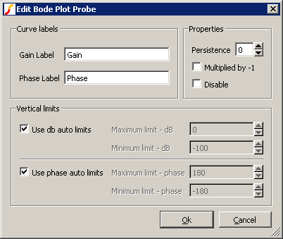
| Options - Bode Plot Probe | |
|---|---|
| Curve labels |
Sets labels for plots
|
| Properties |
Set additional properties on probe:
|
| Vertical Limits |
Divided into two parts to allow setting of axis limits for phase and gain plots.
|
There are currently no fixed probes that create a Fourier Spectrum automatically. Fourier plots can be created manually after the simulation is complete using the procedures described in Fourier Analysis.
Although there are no Fourier fixed probe symbols, it is nevertheless possible to create Fourier plots automatically after the simulation is complete using the simulator's .GRAPH statement and the Spectrum() function. This is added to the F11 window of the schematic. (see Manual Entry of Simulator Commands)
The command to enter in the F11 window is typically of the form:
| .GRAPH "Spectrum(Vector, number_of_points, start_time, end_time)" |
| + curvelabel="curve_label" ylog=y_axis_type |
Where
| Vector | Vector whose Fourier analysis is required. Typically this would be the name of a terminal symbol added to the schematic. (See Finding and Specifying Net Names) |
| number_of_points | Number of sample points used for the Fourier. This must be a power of 2 and will control the maximum frequency in the result. This will be $number_of_points/sample_period/2$ |
| start_time | The start of the sample period in the time-domain data (i.e. transient analysis result) |
| end_time | The end of the sample period in the time-domain data. The best results will be obtained if start_time and end_time define a span that represents a whole number of cycles |
| curve_label | Descriptive label |
| y_axis_type | Set to log for a logarithmic y-axis or lin for a linear axis. |
The above definition shows a typical usage but more options are available. The .GRAPH statement has many more optional parameters and further pre and post processing of the spectrum may be performed. The result can be expressed in dB by applying the dB function:
| .GRAPH "db(Spectrum(Vector, number_of_points, start_time, end_time))" |
| + curvelabel="curve_label" ylog=lin |
A logarithmic x-axis can be specified:
| .GRAPH "Spectrum(Vector, number_of_points, start_time, end_time)" |
| + curvelabel="curve_label" ylog=log xlog=log xmin=start_freq xmax=end_freq |
For more information refer to the Script Reference Manual/Function Reference for details on other functions that can be used in the expression and the Simulator Reference Manual/Command Reference/.GRAPH for details about the .GRAPH statement.
The update period of all fixed probes can be changed from the Options dialog box. Select menu and click on the Graph/Probe/Data analysis tab. In the Probe update times/seconds box there are two values that can be edited. Period is the update period and Start is the delay after the simulation begins before the curves are first created.
|