DVM Tutorial: 6.6.2 Using the ArbitraryCurve() Function

6.6.2 Using the ArbitraryCurve() Function

The ArbitraryCurve() function allows you to generate a curve from an arbitrary mathematical expression of node-voltage and branch-current waveforms. Additionally, the arbitrary mathematical expression can include built-in vector functions, which are all described in Function Reference.

The syntax of the ArbitraryCurve() function has the following syntax with the arguments explained in the table below:

ArbitraryCurve(vector_expression, vectors_to_keep, curve_name, graph_name, grid_index, axis_name, OPTIONAL_PARAMETER_STRING)

Argument	Description
vector_expression	A mathematical expression of node-voltage and branch-current waveforms. This expression can include built-in vector functions.
vectors_to_keep	A space-delimited list of vectors from the vector expression that the program produces in the .PRINT statements for each vector during SIMPLIS simulations and in the .KEEP statements during SIMetrix simulations. This ensures that the vectors supplied in vector expressions are available for plotting after the simulation is complete.
curve_name	Name of the curve that appears next to the graph
graph_name	Name of the graph for the new test report*
grid_index	Grid on which to place the curve*
axis_name	Axis on a particular grid*
OPTIONAL_PARAMETER_STRING	A space-separated set of KEY=VALUE pairs that defines additional formatting parameters**

* For additional information about graph_name, grid_index, and axis_name, see Graph Address System.

** For additional information about OPTIONAL_PARAMETER_STRING, see Optional Parameters.

To plot the AC-coupled output voltage for a converter, follow these steps:

Open the schematic from SIMPLIS_dvm_tutorial_examples.zip at this path: LTC3406B/4.1_LTC3406B - DVM ADVANCED.sxsch.

To assign a net name to the converter output, use the keyboard shortcut y, or from the parts selector, choose Connectors|Terminal.

Place the terminal to the right of the DVM OUT probe and add a connecting line.

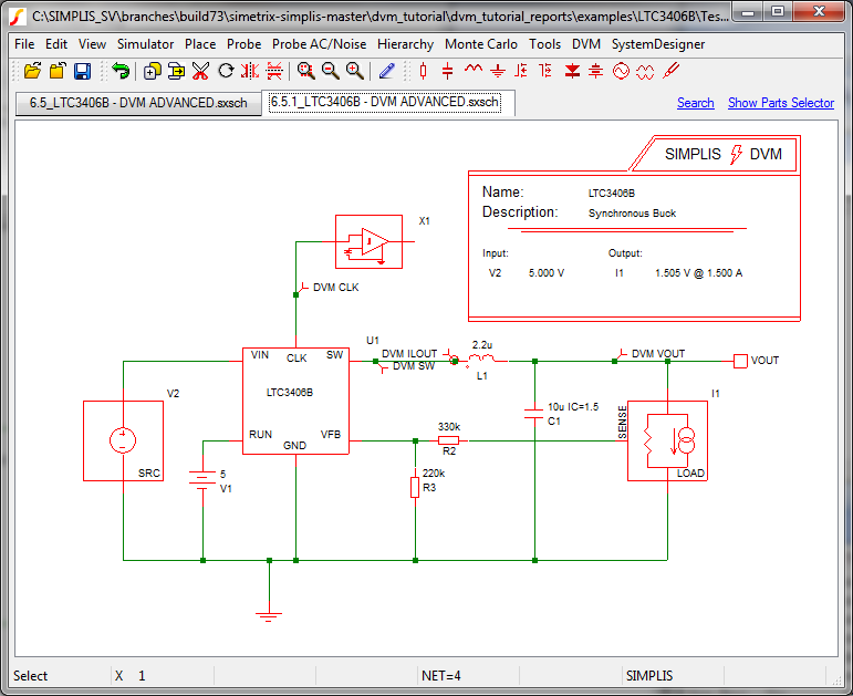
Result: After making this schematic change, the output voltage net will be named #VOUT. The schematic should now look similar to the following, which is available from SIMPLIS_dvm_tutorial_examples.zip at this path: LTC3406B/6.6.2_LTC3406B - DVM ADVANCED.sxsch.

To set up the testplan to generate a curve during a steady-state test objective that runs a POP simulation, follow these steps:

Open the testplan from SIMPLIS_dvm_tutorial_examples.zip at this path: testplans/6.6.1_arbitrary_curve_start.testplan.

Result: This testplan has one test from the built-in sync buck testplan ad looks like the following:

***
*** modified testplan for arbitrarycurve DVM tutorial section 6.6.1
***
*?@ Analysis	Objective	Source	Load	Label
***
Steady-State	Steady-State	SOURCE(INPUT:1, Maximum)	LOAD(OUTPUT:1, 100%)	Steady-State\|Steady-State\|Vin Maximum\|100% Load

Note: Although this testplan has only one test, after you define the curve function, you can copy it to other tests and to other testplans.

In this testplan, add another column and in the header row of the new column, type Create.

Enter the following function into the new Create column, noting the parameters and values in the table below:
ArbitraryCurve(#VOUT-mean(#VOUT), #VOUT, DVM VOUT-AC, default, A4, VOUT-AC)

Argument	Value / Notes
vector_expression	#VOUT - Mean(#VOUT) Note: This is the mathematical expression for the AC coupled output voltage that uses the Mean() vector function to return the average value of the supplied vector over the entire simulation time.
vectors_to_keep	#VOUT
curve_name	DVM VOUT-AC
graph_name	default
axis_name	VOUT-AC (or any other name you prefer)

Result: The testplan should now look like the following with the changes in red. This testplan is available from SIMPLIS_dvm_tutorial_examples.zip at the following path: 6.5.1_arbitrary_curve_final.testplan.

***
*** final testplan for arbitrarycurve DVM tutorial section 6.6.1
***
*?@ Analysis	Objective	Create	Source	Load	Label
***
Steady-State	Steady-State	ArbitraryCurve(#VOUT-mean(#VOUT), #VOUT, DVM VOUT-AC, default, A4, VOUT-AC )	SOURCE(INPUT:1, Maximum)	LOAD(OUTPUT:1, 100%)	Steady-State\|Steady-State\|Vin Maximum\|100% Load

To run the testplan from the schematic, follow these steps:

Open the schematic from SIMPLIS_dvm_tutorial_examples.zip at this path:
LTC3406B/6.6.2_LTC3406B - DVM ADVANCED.sxsch

Select DVM ▶ Run ▶ Choose Testplan... from the main menu of the schematic editor.

Navigate to the testplans directory where you extracted SIMPLIS_dvm_tutorial_examples.zip, and select 6.6.1_arbitrary_curve_final.testplan.

Result: The test report shows a fourth curve on the default graph with the same amplitude and frequency as the VOUT curve, but the vertical axis has a different scale and is centered on zero.

This is one example of the ArbitraryCurve() function. Another version of the function generates X-Y plots. The testplan syntax documentation includes an example where the forward current and forward voltage of a diode are plotted against each other. For more information, see ArbitraryCurve() in the DVM testplan documentation.