Advanced SIMPLIS Training

1.0.1 SIMPLIS is a Time-Domain Simulator, all the Time, for Every Analysis, Period

In this Topic ShowHide

What You Will Learn

How SIMPLIS analyzes circuits exclusively in the time domain.

Getting Started

Exercise #1: Running SIMPLIS

In this exercise, you will simulate a self-oscillating flyback converter in the each of the three SIMPLIS analyses, Periodic Operating Point, AC analysis and Transient Analysis.

1. Open the schematic titled 1.1_SelfOscillatingConverter_POP_AC_Tran.sxsch.

2. Press F9 or use the schematic menu Simulator ▶ Run.
   Result: The SIMPLIS simulator simulates the same time-domain nonlinear schematic in each of the three analysis modes, Periodic Operating Point (POP), AC, and Transient. The SIMPLIS Status window opens when the simulation is first launched, and the graph viewer displays the simulation results. The results from the POP analysis are not displayed, as the transient analysis was specified. Transient results over-write the POP results for all simulations where both POP and Transient are specified. The simulation results displayed in the graph viewer can include waveforms plotted versus time as well as time-domain waveforms that are plotted against each other using X-Y plots, where time in an implicit variable.
   

Discussion

SIMPLIS runs these three analyses in the following order (you will see later in the module that this order is fixed for good reasons):

1. Periodic Operating Point Analysis
2. AC Analysis
3. Transient Analysis

Each of these analyses are executed in the time domain, exactly like what happens on the lab bench. The Periodic Operating Point analysis is discussed in detail in section 1.0.5 POP analysis, for now think of the Periodic Operating Point analysis as a way to accelerate the process of getting to steady state. A key point to remember is that without the Periodic Operating Point, you cannot run an AC analysis on the circuit.

After running the simulation, the graph viewer contains a number of graphs. The first, or left-most tab will have the gain and phase of the converter control loop taken from the AC Analysis. The other tabs will have the results of the transient analysis.

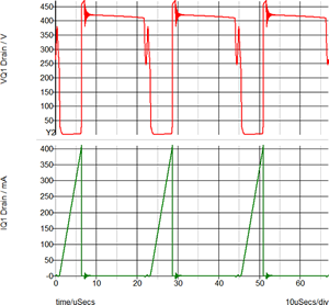
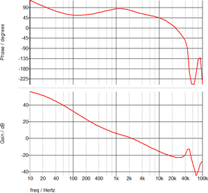
The AC analysis is carried out on the time domain model by first finding the Periodic Operating Point, then injecting a single time-domain sinusoidal perturbation signal into the circuit. The AC results are then calculated from the time domain response of the perturbation signal, and the next frequency to be analyzed is injected and the measurement process repeats. No averaged model is used. The time domain POP waveforms and the frequency-domain loop response of the Self-Oscillating Converter are shown below. You can click on each image to view an enlarged image.

The transient analysis is similar to a transient analysis in other simulators, except it typically runs much faster.

Conclusions and Key Points to Remember

SIMPLIS operates just like your circuit in the laboratory - in the time domain.

• Your power electronic switching system in the lab has no concept of a DC operating point or an AC model.
• The power switches turn ON and then OFF as determined by a modulator control circuit that senses the output and tries to regulate the circuit performance accordingly.
• If the circuit is not switching, it is not working correctly.
• A switching converter has no DC operating point.
• An averaged AC model is a theoretical construct, it does not exist on the lab bench.
• If you cannot successfully perform a POP analysis on your circuit:
• 1. You cannot easily evaluate the AC performance of the circuit. ( Caveat: DVM has a multi-tone AC analysis, but this takes much longer than the combination of a POP and AC analysis. )
  2. In the vast majority of cases, your simulations will take much longer, since you will have to first wait for the converter to reach steady state before you can perform your intended analysis.

Reference Material

• SIMetrix/SIMPLIS help system topic : What is SIMPLIS? ▶ SIMPLIS - Time Domain, All the Time

© 2015 simplistechnologies.com | All Rights Reserved