Advanced SIMPLIS Training

1.0.2 PWL Simulation and Modeling

In this Topic ShowHide

What You Will Learn
Getting Started
Discussion
SIMPLIS Primitive PWL Models
Conclusions and Key Points to Remember
Reference Material

What You Will Learn

Every device model used in a SIMPLIS simulation uses Piecewise Linear (PWL) modeling techniques.

Getting Started

This topic picks up where topic 1.0.1 leaves off. After the simulation completes, the graph viewer displays multiple graph tabs. If you have closed the graph viewer or one of the graph tabs, run the simulation again to regenerate the graphs. The right-most two graphs are of interest, these two graph tabs will be similar to:

Discussion

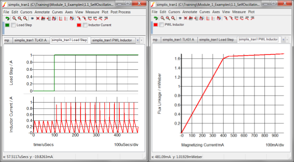
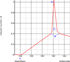
The left hand graph contains two curves, the Load Step in green, and the Magnetizing Inductor Current in red.

During the transient simulation, a one amp load step is applied at 100us. During this load step, the total load current transitions from a 2A full load condition to a 3A overload condition with the consequence that the transformer enters into saturation. The current limit function is triggered and the output voltage drops. The following graph is zoomed in on the first 200us of the simulation.

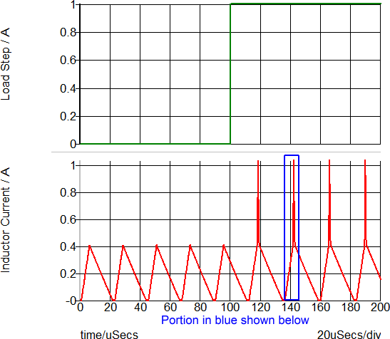
This overload condition demonstrates how a PWL inductor models the saturation of a transformer magnetizing inductance. The following two graphs show a close-up view of the time-domain magnetizing inductor waveform and the flux linkage versus current plane on which PWL inductors are defined. Each of these three PWL inductor segments can be seen in both the transient simulation results and in the x-y plot of the flux linkage versus current plane show below:

Magnetizing Current and B-H Loop for Self-Oscillating Converter
Saturating Magnetizing Current	B-H Loop

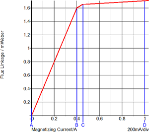The saturation of this transformer is modeled with three PWL segments in the flux linkage versus current plane. Because the slope of this curve is the magnetizing inductance, the magnetizing inductance can take on three distinct values:

When the magnetizing current is below 0.4A, the normal or unsaturated magnetizing inductance of 1.6mWeber/0.4A equals 4mH is used.
The knee of saturation occurs when the magnetizing current is between 0.4 and 0.45A. The inductance in this region is (1.65m-1.6m)/(0.45-0.40) which equals 1mH.
The final PWL segment represents a "hard" saturation. The inductance of this segment is 100uH.

What about the Diodes or the MOSFET on the schematic? Are these PWL models as well? Yes!

In SIMPLIS, the built-in diode models are nothing more than PWL resistors with either 2 or 3 segments. The PWL definition is usually generated with the automatic model parameter extraction routines built into SIMetrix/SIMPLIS.
The built-in MOSFET models are made from a collection of PWL devices, including:
- A PWL resistor representing the body diode
- A transistor switch with a constant forward transconductance gain (Gm)
- PWL capacitors representing the voltage dependent nonlinear capacitance effects

As an example, the output rectifier in Self-Oscillating Converter has the following Forward Current and Forward Voltage curves during the transient simulation. The left hand graph has the Forward Current and Forward Voltage plotted vs. Time. In the right-hand graph, the Forward Current is plotted versus the Forward Voltage for this diode. The Blue curve is the 3 segment SIMPLIS PWL model. The red curve is the SIMetrix simulation results for SPICE model of the same diode.

Output Rectifier Voltage and Current
Voltage and Current vs. Time	Voltage vs. Current

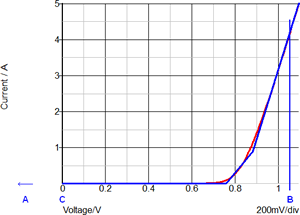The annotated points describe the following diode states:

Blocking state
Conducting 4A forward current
Transition from conduction to blocking state

An in depth discussion of MOSFET modeling is presented in section 1.0.4 Multi-Level Modeling.

SIMPLIS Primitive PWL Models

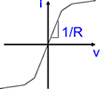
The table below illustrates how SIMPLIS represents PWL resistors, PWL capacitors, and PWL inductors as a set of PWL straight-line segments. A PWL resistor is piecewise linear in the current versus the voltage plane. The slope of this curve is the conductance. SIMPLIS automatically extends the left-most and right-most PWL segment to negative and positive infinity, respectively.

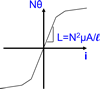
PWL capacitors are defined on the charge versus voltage plane where the slope is capacitance. PWL inductors are defined on the flux-linkage versus current plane, where the slope is inductance. The units of flux linkage are Weber-Turns or volt-seconds.

PWL Resistor	PWL Capacitor	PWL Inductor


x-value ⇒ Voltage	x-value ⇒ Voltage	x-value ⇒ Current
y-value ⇒ Current	y-value ⇒ Charge	y-value ⇒ Flux Linkage
Slope=1/Resistance	Slope=Capacitance	Slope=Inductance

Conclusions and Key Points to Remember

Every device used in a SIMPLIS simulation, behind the scenes, is a PWL model. This is independent of the symbol. The symbol is merely a graphical representation of the underlying function being modeled.
The nonlinear characteristics of Resistors, Capacitors, and Inductors are modeled as a series of PWL straight line segments.
Even complex devices, such as MOSFETs can be represented by a collection of PWL devices.

Reference Material

SIMetrix/SIMPLIS help system topic : What is SIMPLIS? ▶ SIMPLIS - Piecewise Linear, All the Time

◀ 1.0.1 SIMPLIS is a time-domain simulator, all the time, for every analysis, period

1.0.3 Accuracy of PWL models ▶