Advanced SIMPLIS Training

To download the examples for Module 2, click Module_2_Examples.zip

2.3.2 The Core POP Process

In this Topic ShowHide

What You Will Learn

1. The Core POP Process recursively calculates and refines the initial conditions of the system, causing the circuit to reach steady-state much faster than running a long transient.

2. The details of a "pass" through the Core POP Process.

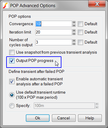
3. The progress of a POP analysis can be output to the graph viewer by checking the Output POP progress check box on the POP Advanced Options dialog.

 Getting Started

Exercise #1: POP Advanced Options

1. Open the schematic 2.7_SelfOscillatingConverter_POP.sxsch.

2. From the schematic menu, select Simulator ▶ Choose Analysis... menu option. The training material shortcut F8 will execute this menu item.
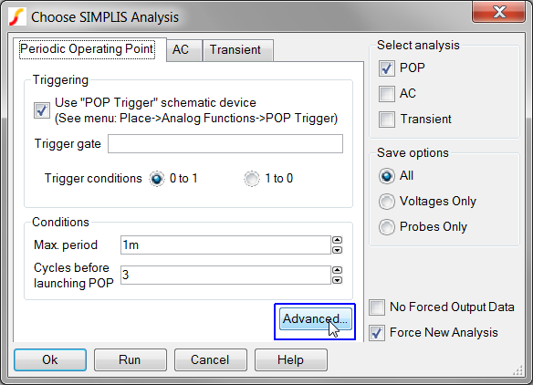
   Result: The Choose Analysis dialog opens to the POP tab.

3. Click on the Advanced... button to open the POP Advanced Options dialog.
   
   Result: The POP Advanced Options dialog opens:
   

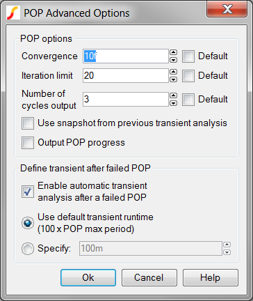
4. Check the Output POP progress check box. The dialog should now appear as follows:
   

5. Click the Ok button on the POP Advanced Options dialog.

6. Click the Run button on the Choose SIMPLIS Analysis dialog.
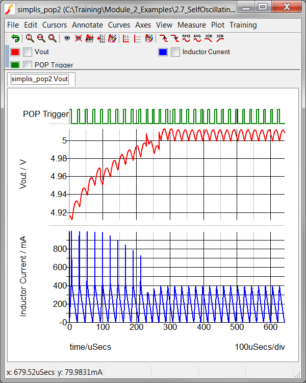
   Result: The POP simulation starts and as the simulation progresses, the output voltage waveform, Vout, has vertical discontinuities, or jumps, where the Core POP Process predicts and sets the initial conditions of the circuit.
   

Discussion

POP Data in the Time Domain

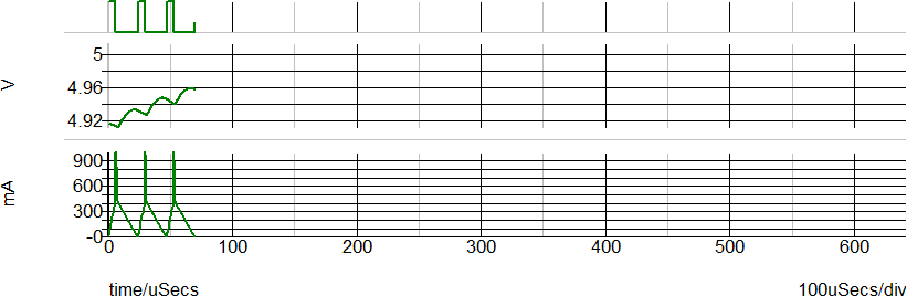
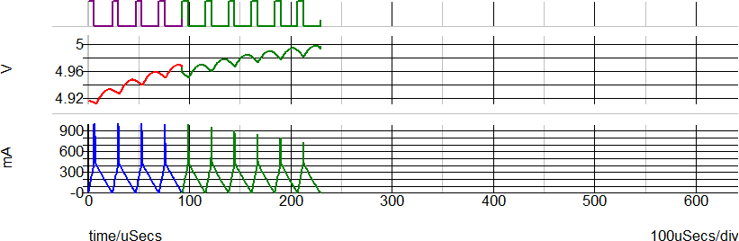
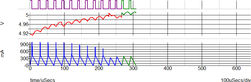
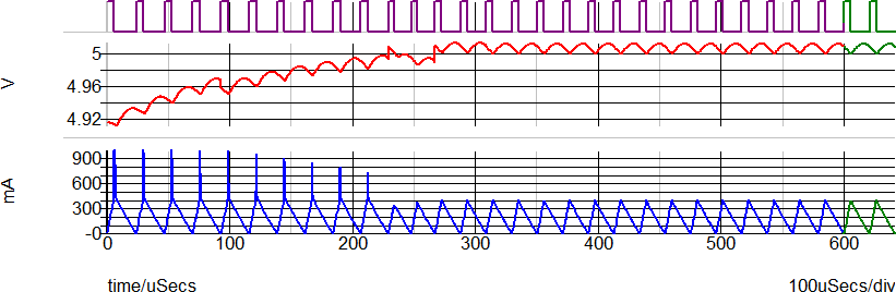
In the previous topic, 2.3.1 Overview of the POP Analysis, the POP Analysis was divided into four phases, labeled A-D. In the simulation you ran in the Getting Started section of 2.3.1 Overview of the POP Analysis, the graph viewer displayed 3 cycles of steady-state operation from phase D of the POP Analysis. In the getting started step of this topic, you instructed SIMPLIS to show all intermediate simulations which were generated to bring the converter to steady state, that is, all simulation data generated in phases A-C of the POP analysis. Using the same phase notation from the previous topic, a graph annotated with each phase of the POP analysis for this converter is shown below:

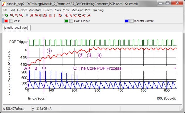
In this graph, it is easy to see how the majority of the time spent in the POP Analysis occurs during the Core POP Process. The Core POP Process is a sequence of short transient simulations, where a new set of circuit initial conditions is calculated prior to each transient simulation. In the above graph, the purple numerals 1-4 annotate the first four times that the POP algorithm calculated a new set of initial conditions. Although the circuit initial conditions are recursively calculated and set at the beginning of each pass through the POP Process, the changes for the remaining POP passes are so small that they cannot be visually detected on the graph. Each of these initial condition reset events initiates a pass through the Core POP Process.

Core POP Process Flow Chart

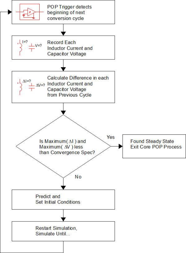
The Core POP Process is essentially a software control loop applied to your circuit. As such, the Core POP Process can be described with the flow chart below. In this flow chart, each POP "Pass" or interation represents a complete loop through the flow chart. When the circuit reaches steady-state, the Core POP Process is exited and the simulator generates the Number of cycles output from Phase D of the POP Analysis described in 2.3.1 Overview of the POP Analysis.

Note: The number of actual switching cycles simulated per pass through the POP Process is variable.

POP Data Presented on the State Plane

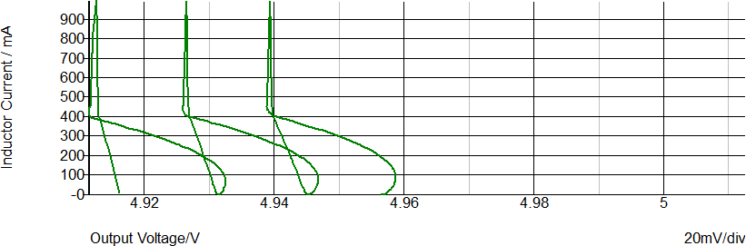
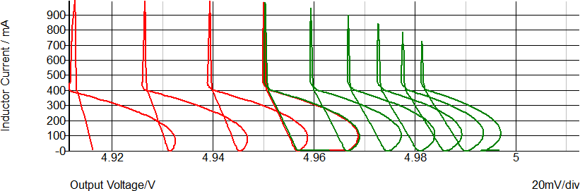
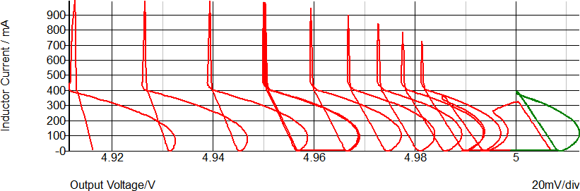
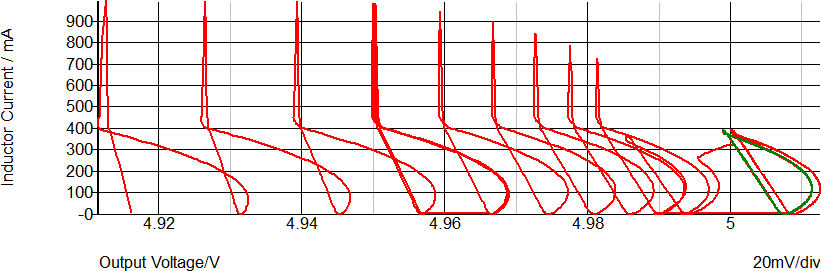
The flyback converter used in example 2.7_SelfOscillatingConverter_POP.sxsch has two main energy storage elements, the magnetizing inductance L4, and the output capacitance C1. A state plane plot is nothing more than a x-y plot of the inductor current vs. the capacitor voltage. The state plane plot of the two main energy storage elements of the converter is often useful to visualize the response of the converter. In the next exercise, you will output a state plane plot for the converter.

Exercise #1: Generate a State Plane plot

1. Close the graph viewer.

2. On the upper right hand corner of the schematic find the XY probe connected to the output:
   

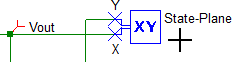
3. Double click on the probe to open the Edit Probe dialog. Un-check the All analyses disabled check box as show below:
   
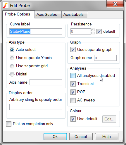
   Result: Both the POP and Transient analysis check boxes will be checked.

4. Click Ok to accept the Edit Probe dialog changes.

5. Run the simulation.
   Result: The simulation executes as before, showing the POP progress. After the simulation completes, the x-y state plane plot is generated.
   

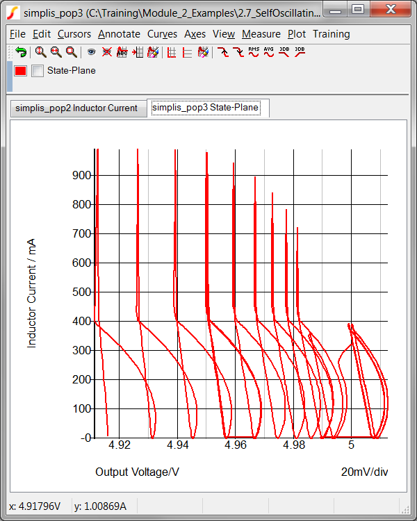
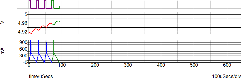
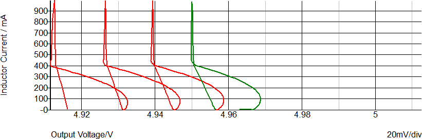
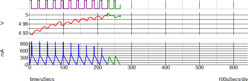
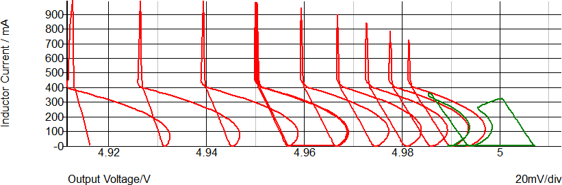
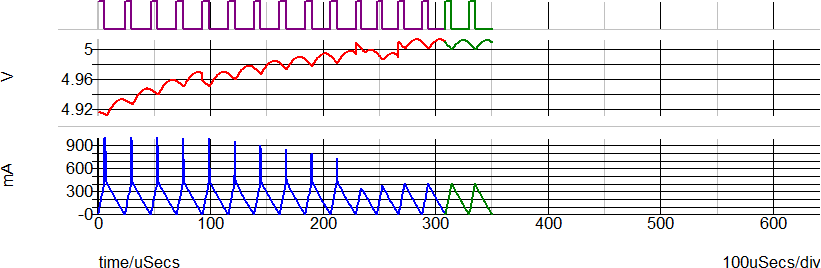
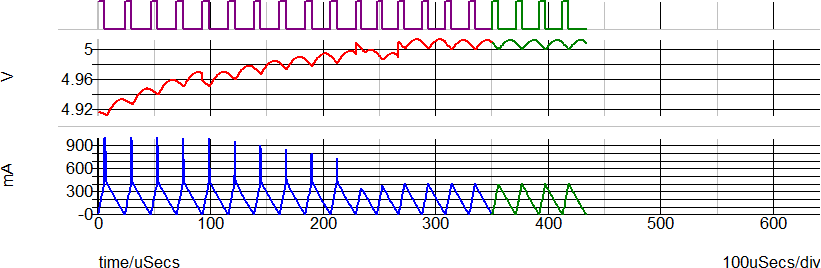
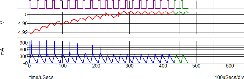
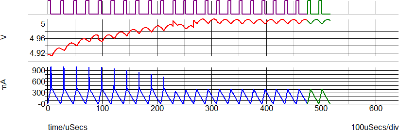
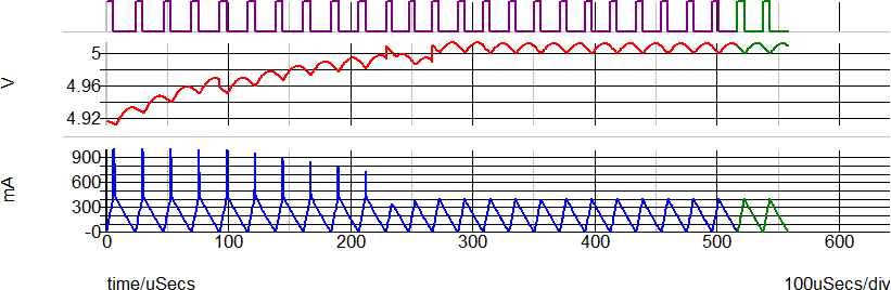
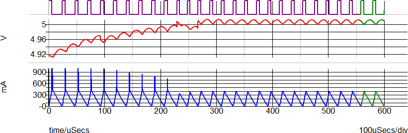
Notice that the time variable doesn't appear in the state plane plot. To better visualize how the converter enters into steady state, you have taken the same simulation results and overlaid green curves representing the different passes through the Core POP Process. In the animated GIF image below, the actual simulated output voltage and magnetizing current, as well as the state plane plot are plotted.

Animated Core POP Process

The following slideshow illustrates the sequence of actions that occur during a POP analysis.

• You can pause the slideshow by moving the mouse cursor over the images.
• To go forward or back one slide, click the arrow links that appear when you mouse over the slideshow.
• Each slide number is shown in the bottom right-hand corner. You can jump to a particular slide by clicking one of the gray squares at the bottom on the image. The current slide is indicated by the white square.

 

 

1 of 12

Cycles Before POP

2 of 12

PASS: 1

3 of 12

PASS: 2

4 of 12

PASS: 3

5 of 12

PASS: 4

6 of 12

PASS: 5

7 of 12

PASS: 6

8 of 12

PASS: 7

9 of 12

PASS: 8

10 of 12

PASS: 9

11 of 12

PASS: 10

12 of 12

PASS: 11

 

 

POP Advanced Options Dialog

Most parameters for the Core POP Process are set on the POP Advanced Options dialog, shown below with annotations:

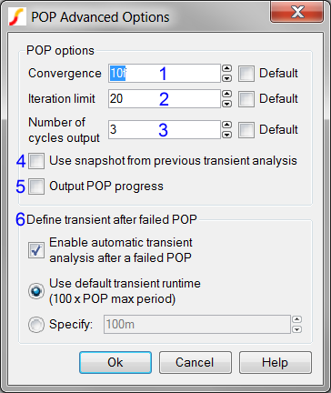	1: The maximum change in any state element when the circuit is in steady-state.
	2: The maximum number of passes through the Core POP Process.
	3: The number of steady-state cycles to output to the graph viewer.
	4: If checked, the POP analysis will start using a snapshot from a previous transient analysis.
	5: If checked, the graph will display the POP Progress instead of the steady-state Number of cycles output.
	6: Determines the behavior if the POP analysis fails.

Conclusions and Key Points to Remember

• Each Pass through the Core POP Process calculates a new set of initial conditions for each state variable, performs a time-domain simulation of the system for an integer number of switching cycles, and measures the change in each state variable from one conversion cycle to the next. The system is considered to be in steady state once the magnitude of change in each of the state variables is less than the convergence criteria.
• The Core POP Process recursively calculates and refines the initial conditions of the system, causing the circuit to reach steady-state much faster than running a long transient.
• You can view the Core POP Process progress by checking the Output POP progress check box on the POP Advanced Options dialog.

© 2015 simplistechnologies.com | All Rights Reserved