Advanced SIMPLIS Training
Advanced SIMPLIS Training
|
To download the examples for Module 2, click Module_2_Examples.zip
In this Topic Hide
SIMPLIS saves switching instance data, or topologies, during the simulation
What a "new topology" is
Basic and Advanced Transient Analysis Settings
Force New Analysis and Transient Snapshots
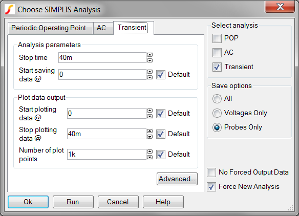
Open the schematic titled 2.1_SelfOscillatingConverter_Tran.sxsch from the Module_2_Examples.zip file. This is the same circuit used in section 1, but with only two probes enabled and with different analysis settings.
From the schematic menu, select Simulator
Choose Analysis... The training
material shortcut F8 will
execute this menu item.
Result: The Choose Analysis dialog opens
to the Transient tab:
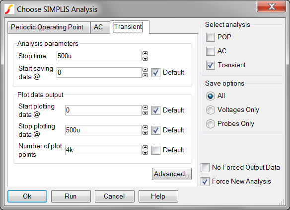
The SIMPLIS Transient analysis settings are divided into two groups:
There is a distinct difference between the Analysis parameters and the Plot data output parameters. The Analysis parameters, in particular the Stop time, define the time interval which SIMPLIS will collect switching instance data. Switching instance data is the state of each topology as the circuit switches from one PWL topology to the next. The switching instance data is internal to SIMPLIS and is not output to the graph viewer as vectors.
The Plot data output parameters define which time slice of switching instance data is translated to analog and digital vectors for plotting on the graph viewer. The Plot data output parameters can be set to limit the time span of the output data.
During a SIMPLIS simulation, the PWL circuit will repeatedly change between multiple unique PWL topologies. For example, in a typical flyback converter, there exists an energy storage phase where energy is extracted from the source and stored in the magnetic field of the transformer. This is followed by a flyback phase where this stored energy is delivered to the load. This simple example represents two PWL topologies. As the SIMPLIS simulation progresses, SIMPLIS identifies these topologies and stores the topology information for later use. The first time a unique topology is encountered, SIMPLIS declares this to be a "new topology." In plain terms, SIMPLIS learns the circuit as the simulation progresses.
Because SIMPLIS stores these topologies for future use, and it takes some computational power to store and retrieve the topology information, the more topologies a circuit transitions through, the slower the SIMPLIS simulation will be. In this section only the Transient analysis is considered and a simple circuit is used as an example.
A few exercises will bring these points home. Throughout these exercises keep in mind that the number of new topologies is one factor which slows down a SIMPLIS simulation. Since the example circuit is fairly small, the execution time will be dominated by factors other than the number of topologies. However; as circuit size increases, the number of new topologies becomes a key consideration. For these reasons, the exercises will focus on the number of new topologies rather than the actual simulation execution time.
A baseline simulation which can be compared with exercise results is required. To run a baseline simulation,
Click Cancel on the Choose Analysis dialog.
Open the SIMPLIS Status Window. The training keyboard shortcut Ctrl+Space will bring the window into focus.
Clear the messages by clicking on the "Clear Messages" button.
Press F9 to run the simulation
Result: SIMPLIS runs the transient analysis
on the circuit, the SIMPLIS Status window shows the progress of the
simulation.
During the 500us simulation time, the circuit transitions through 185 new topologies. Look in the SIMPLIS status window (Ctrl+Space) for the point where the simulation was 50% complete:
41 42 43 44 New topology #174
45 46 47 48 49 50
51 52 New topology #175
There were 174 new topologies encountered from the start of the simulation until the simulation time reached 250us, which is 50% of the Stop time.
Now, lets change the stop time to 250u, and rerun the simulation.
From the schematic menu, select Simulator
Choose Analysis... The training
material shortcut F8 will execute this menu item.
Result: The Choose Analysis dialog opens
to the Transient tab.
Change the stop time to 250u as shown below:
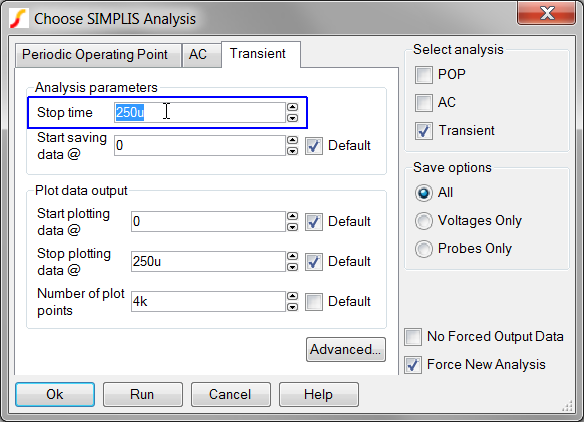
Press F9 to run the simulation.
Result: the simulation runs to 250us. The
number of new topologies is 174, as expected.
81 82 83 84 85 86 87 88 New topology #174
89 90
91 92 93 94 95 96 97 98 99 100
Conclusions from Exercise #1:
The number of new topologies depends on the simulation Stop time.
A higher quantity of new topologies occur in the beginning of the simulation. As SIMPLIS learns the circuit, fewer new topologies are found and saved. In the experiment you decreased the simulation Stop time by a factor of two, and the topologies only changed from 185 to 174.
In the next exercise you will change the Start saving data parameter, and see how this changes the number of new topologies.
Now, lets change the Start saving data time to 50u, and rerun the simulation.
Close the graph viewer.
Open the SIMPLIS Status Window. The training keyboard shortcut Ctrl+Space will bring the window into focus.
Clear the messages by clicking on the "Clear Messages" button.
From the schematic menu, select Simulator Choose Analysis... The training material shortcut F8 will execute this menu item.
Change the stop time to Start
saving data @ time to 50u as shown below:
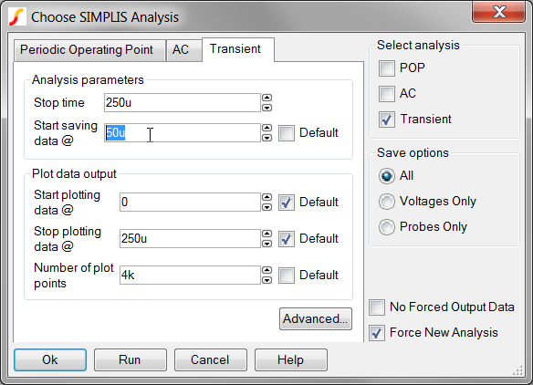
Result: The simulation executes and 174 new topologies are found before the simulation completes. This is the same number of new topologies you found in the previous exercise. The graph viewer displays the simulation results from 50u to 250us.
81 82 83 84 85 86 87 88 New topology #174
89 90
91 92 93 94 95 96 97 98 99 100
Conclusion: The number of new topologies does not depend on the Start saving data @ time parameter. This is expected because SIMPLIS simulates the circuit from time equals zero. Each new topology encountered is saved for future use.
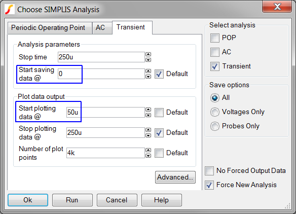
Now lets change the Start plotting data time to 50u, and rerun the simulation. You will also reset the Start saving data time to the default, which is zero.
Close the graph viewer.
Open the SIMPLIS Status Window. The training keyboard shortcut Ctrl+Space will bring the window into focus.
Clear the messages by clicking on the "Clear Messages" button.
From the schematic menu, select Simulator Choose Analysis... The training material shortcut F8 will execute this menu item.
Check the default check box next to the Start saving data @ time.
Change the Start plotting data
@ time to 50u as shown below:
Run the simulation.
Result: The simulation executes and, as with the previous experiment, 174 new topologies are encountered before the simulation completes. The graph viewer displays the simulation results from 50u to 250us.
Next you will learn about the Force New Analysis check box, and how this option affects the simulation.
At this point you know SIMPLIS has the ability to very closely save the state of the circuit for future use. By default SIMPLIS saves the state, or Snapshot, of the PWL circuit at time=0 and at the Stop time. These two snapshots are always available for use in a future simulation. In the previous exercises, you have told SIMPLIS to ignore any previous state information by checking the Force new analysis check box.
Consider the following real-world simulation situation:
You are developing a PFC controller and would like to closely examine the startup behavior of the circuit. Your first task is to examine the first two complete line cycles (40ms at 50Hz Line), then move onto the successive line cycles. Since PFC converters are switching at a high frequency and have a line frequency input which is much lower frequency, these converters are computationally intensive. To save time, it would be nice to be able to store the state after any number of line cycles and pick up that state in a future simulation. This is exactly how SIMPLIS works.
An exercise will demonstrate loading the simulation state. To get started,
Close all open schematics without saving.
Open the example 2.2_PFC_Critical_Conduction_Mode.sxsch from the Schematic menu Training Module 2 2.2_PFC_Critical_Conduction_Mode.sxsch menu.
Close the graph viewer.
Open the SIMPLIS Status Window. The training keyboard shortcut Ctrl+Space will bring the window into focus.
Clear the messages by clicking on the "Clear Messages" button.
From the schematic menu, select Simulator
Choose Analysis... The training
material shortcut F8 will
execute this menu item.
These default analysis settings will ignore previous Snapshot information,
and will simulate from 0 to 40ms.
Run the simulation.
The simulation will take approximately 15-20 seconds to complete. The graph viewer will open to display the control signals:

Now you will tell SIMPLIS to load the state of the PFC circuit at 40ms, and continue to simulate for another 60ms to the stop time of 100ms.
From the schematic menu, select Simulator Choose Analysis... The training material shortcut F8 will execute this menu item.
Make the following changes to the dialog:
Un-check the Force New Analysis check box.
Set the Stop time to 100m.
Set the Start saving data
to 40m.
The configured dialog should appear exactly
as follows:
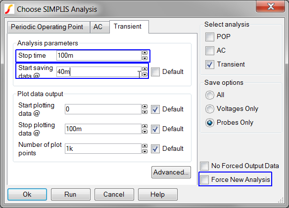
Double check the dialog appears exactly as above. You will not get a second chance if the analysis settings are incorrect.
Run the simulation by clicking on the Run button.
Result: SIMPLIS loads the state of the
simulation at 40ms, and simulates to 100ms.
The graph viewer now shows two sets of curves, one each from each simulation run. The second simulation starts where the first simulation left off, at 40ms.

If you look carefully in the SIMPLIS Status window, you will see a message (you may have to scroll up to find the message near the top):
Reading the state/snapshot of the simulation at t = 4.00000000e-002 sec
This message indicates that at the start of the transient analysis, SIMPLIS has loaded the previous Snapshot information at time=40ms
A number of items will prevent SIMPLIS from loading snapshot information:
There is no previously saved snapshot information to load.
The Force new analysis check box is checked.
The circuit has materially changed since the last snapshot was taken.
No snapshot is available to load because of the analysis parameter settings. This will be explained next.
In this exercise two snapshots are available from the first run, one at time=0 and one at the Stop time of 40ms. What happens if you re-run the simulation with the Start saving data parameter set to 39ms, which is 1ms prior to your last saved Snapshot? Lets try it.
From the schematic menu, select Simulator Choose Analysis... The training material shortcut F8 will execute this menu item.
Open the SIMPLIS Status Window. The training keyboard shortcut Ctrl+Space will bring the window into focus.
Clear the messages by clicking on the "Clear Messages" button.
Change the Start saving data parameter to 39ms. You will have
to select the 40m value in the spin box and type 39m.
The dialog should appear as follows:
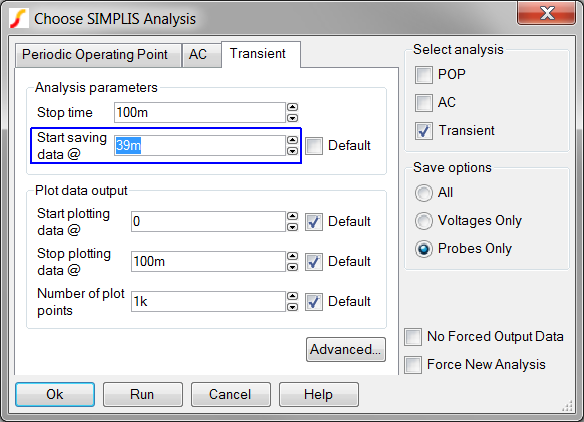
Run the simulation.
The closest Snapshot prior to the 39ms start time is the first Snapshot at time=0. SIMPLIS loads this snapshot and simulates, starting at time=0. SIMPLIS internally stores the switching instance data for the first 39ms, then at time=39ms, starts to output the analog waveforms. The entire simulation will take approximately 35s, because the simulator is effectively starting from time=0.
Its clear a method is require to define more snapshots, so the simulation doesn't have to start at time=0 each time. As it turns out, the Advanced Transient Analysis options offer exactly this functionality.
Clicking on the Advanced.. button will open the Advanced Transient Options dialog:
![]()
To save additional snapshots in between the default Snapshot at time=0 and at the Stop time,
Check the Enable snapshot output
check box.
Result: The Snapshot
interval and Max
snapshots controls are enabled.
Enter the desired snapshot interval in seconds in the Snapshot interval entry.
Enter the maximum number of snapshots in the Max
snapshots entry.
| Caution: The maximum number of snapshots will over-ride your Snapshot interval if a conflict arises. |
( not covered in class )
Go back through exercise numbers 4 and 5 with the Snapshot interval set to 1ms, and the maximum number of snapshots set to 50. Run the first simulation to 40ms, then re-run the simulation loading the Snapshot starting from 39ms.
© 2015 simplistechnologies.com | All Rights Reserved