Advanced SIMPLIS Training
Advanced SIMPLIS Training
|
To download the examples for Module 2, click Module_2_Examples.zip
In this Topic Hide
How and where SIMetrix/SIMPLIS stores simulation data.
How to manage data groups.
How to control the size of the data group.
How to use .KEEP statements to add hierarchical data to the data group.
Close and restart SIMetrix/SIMPLIS.
Open the schematic 2.3_SelfOscillatingConverter_POP_AC_Tran.sxsch using the training menu shortcut.
Run the simulation.
From the command shell menu, select Graphs
and Data Change Data Group...
Result: The Change Groups dialog opens,
displaying which data groups are available: The selected data groups
is the current group.
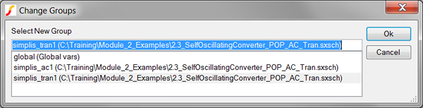
After every POP, Transient, or AC analysis, SIMPLIS stores the simulation results in a data group. Data groups are automatically named according to the analysis type, and to guarantee uniqueness, the group name is appended with an integer. When SIMetrix/SIMPLIS starts, the integer is set to 1, and the integer increments every time you run a SIMPLIS simulation. In the Change Groups dialog above, there are three groups,
As discussed in 1.0.1 SIMPLIS is a Time-Domain Simulator, all the Time, for Every Analysis, Period, the transient simulation over-writes the POP simulation data. So in this example, you ran three simulations and from those three simulations, there are two data groups. The global group contains global variables used in the SIMetrix/SIMPLIS User Interface.
Each data group is completely independent of the other data groups. Each data groups contains the simulation vectors for that simulation, but no information on how those vectors were plotted on the graph viewer. The plot journal method described in the 2.1.6 Using Plot Journals topic records how vectors were plotted and, when the you run the plot journal, the graph is recreated from the vectors in the current data group.
Data groups are stored in files on your local hard drive. Where data groups are saved and when they are deleted is set in the Options/Preferences... dialog. To view or change the location where the data groups are saved,
Cancel the Change Groups dialog.
From the command shell menu, select File Options General...
Select the File Locations tab. The dialog should appear
as follows:
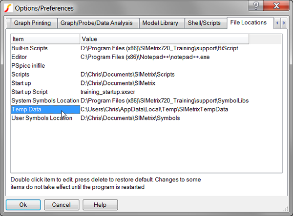
As with the other options, you can select a directory location where the data is saved. To change the directory, double click the Temp Data item.
You can save the Temp Data to any location on your local hard drives.
| Caution: You are strongly discouraged from using a network drive to store your Temp Data. File access times to the data groups are critical for the performance of SIMetrix/SIMPLIS. |
At any time, only one data group is the "current group." The current group is the group which SIMPLIS uses to plot data from the simulation, or if you probe the circuit after the simulation completes. Since you ran a POP then AC, then Transient, the transient run is the current data group. You can change the current group to plot different simulation runs or to compare data using the command shell menu: Graphs and Data Change Data Group...
Data groups can be loaded from disk with the command shell menu File Data Load...
A setting in SIMetrix/SIMPLIS controls when data groups are deleted. In the Options/Preferences dialog, on the Graph/Probe/Data Analysis tab:
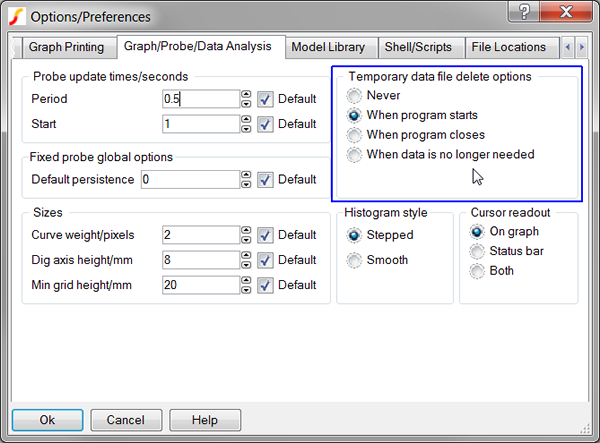
The first three options are self explanatory, only the last option requires discussion. When data is no longer needed retains only the last three data groups. While this is the most aggressive setting, it is almost required for very large circuits or for simulations which are executed in a loop, such as DVM. For more information on this setting click on the Help button on the dialog.
The size of the data group is largely determined by two factors:
The number of vectors is determined by the Save options settings on the Choose Analysis... dialog. Below is the dialog for the 2.3_SelfOscillatingConverter_POP_AC_Tran.sxsch. The Save options group determines how many top level vectors are output to the data group. This setting applies to all analyses.
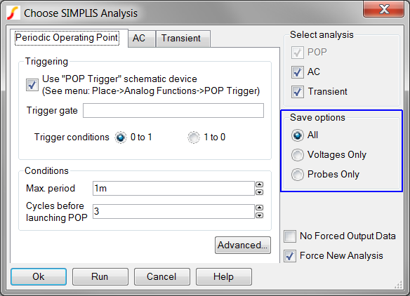
| The Save options applies only to the top level vectors, that is, the vectors on the .sxsch schematic. |
The three Save options apply to the top level circuit only. By default, the only vectors saved in hierarchical blocks are from probes inside those blocks.
To output vectors inside the design hierarchy, you use the .KEEP command in the F11 window of the hierarchical block. The next exercise demonstrates how .KEEP commands work.
Open the schematic 2.3_SelfOscillatingConverter_POP_AC_Tran.sxsch, if it is closed.
Run the simulation.
Select the opto-coupler U1.
Press Ctrl+E to descend into the schematic view for the opto-coupler.
From the schematic menu, select
Probe
Voltage.
 |
Position the probe over the wire connecting the positive pin of C1 and the positive control input to G1.
Press the left mouse button.
Result: Nothing happens!
Something did actually happen - an error message was output to the command shell. The error message output is:
Cannot
plot that node voltage. Possible reasons:
1. No simulation has been run on that schematic
2. The wrong data is selected for that schematic. Use "Graphs And
Data | Change Data group" to select the correct data
3. The data for that node was not saved in that simulation
The reason for the error in this case is the third item: The data doesn't exist for the node which you probed, because you haven't told SIMPLIS to output the data to the data group. To output the voltages on the opto-coupler schematic,
Select the opto-coupler U1.
Press Ctrl+E to descend into the schematic view for the opto-coupler.
Press F11 to open the command window.
There is one commented out command in the F11 window:
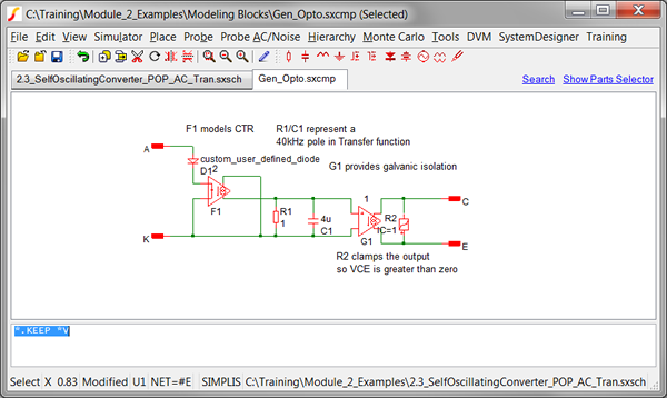
Remove the leading comment character (*) so the statement reads .KEEP *V, and note there is a space between the .KEEP and the *V.
Run the simulation.
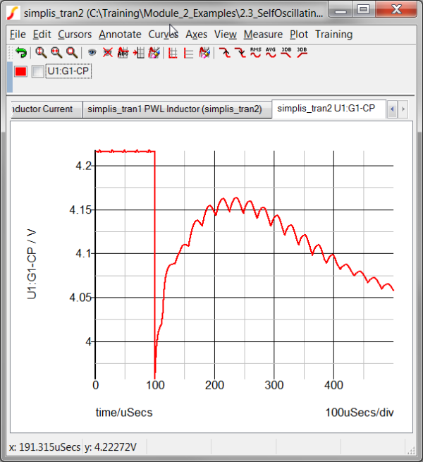
Now, probe the circuit again:
Select the opto-coupler U1.
Press Ctrl+E to descend into the subcircuit for the opto-coupler.
Use the keyboard shortcut Ctrl+R to repeat last probe action.
Click on the positive node of C1.
Result: The graph viewer displays the plot
of the voltage waveform for the transient analysis.
The following guidelines will be helpful to select .KEEP statements
| Command | Action |
.KEEP *V |
Keeps all voltages at this hierarchical level. |
.KEEP **V |
Keeps all voltages at this hierarchical level and all lower levels. |
.KEEP *I |
Keeps all currents at this hierarchical level. |
.KEEP **I |
Keeps all currents at this hierarchical level and all lower levels. |
.KEEP *I **V |
Keeps all currents at this hierarchical level and all voltages at this hierarchical level and all lower levels. |
| Other combinations are possible using a space separated list of voltage and current declarations. | |
| Caution: For large circuits, placing a .KEEP **V at the top level will save an enormous amount of data. Using .KEEP **V **I will save even more data, as all currents will be added to the data group. | |
| Caution: When you package your circuit for encryption and distribution, make certain you do not have .KEEP statements in the hierarchy. Any .KEEP statements will output simulation vectors to the data group, possibly exposing some internal intellectual property. This will be discussed in more detail in the 4.4 Protecting Your Intellectual Property - Model Encryption topic. |
SIMPLIS creates output vectors in an orderly and consistent manner. At every topology change, SIMPLIS will add a data point to each simulation vector. In addition to these points, SIMPLIS adds uniformly distributed points from the simulation start to the simulation stop time. SIMPLIS adds the number of uniformly distributed points defined in the Choose Analysis... dialog on the Transient tab. Below is the transient tab for the 2.3_SelfOscillatingConverter_POP_AC_Tran.sxsch converter.
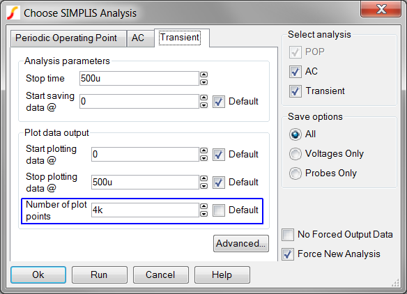
With these settings, SIMPLIS will generate 4000 data points evenly spaced over the 500us simulation time. Additional points will be added every time the circuit changes PWL topologies. The next example will help to better understand this behavior.
Open the 2.3_SelfOscillatingConverter_POP_AC_Tran.sxsch schematic.
Close the Graph Viewer.
Run the simulation.
Result: SIMPLIS Runs POP, AC and Transient
simulations. The current data groups contains the simulation vectors
from the last analysis, that is the Transient simulation.
On the graph viewer, select the Inductor Current tab.
Select the Inductor Current
curve on the curve legend.
Result: The check box to the left of the
curve name is checked.
From the graph menu, select Training
Show Vector Len of Sel Curves.
Result: The command shell contains a message
with the length of the Inductor Current curve vector.
In the command shell will be a message:
length = 5632
This message tells us the Inductor Current vector contains 5632 data points.
Press F8 to open the Choose Analysis... dialog.
Select the Transient tab.
Change the Number of plot points
to 1. The dialog should appear as follows:
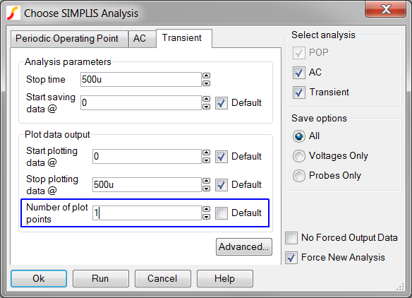
Run the simulation.
On the graph viewer, select the Inductor Current tab.
De-Select the Inductor Current curve from the first simulation. This curve should be Red.
Select the new Inductor Current curve. This curve should be
green and have a (simplis_tran) after the curve name on the graph
legend.
Result: The check box to the left of the
Inductor Current curve name is checked.
From the graph menu, select Training
Show Vector Len of Sel Curves.
Result: The command shell contains a message
with the length of the Inductor Current curve vector.
In the command shell will be a message:
length = 1634
This message tells us the Inductor current vector contains 1634 data points. Note this is 3998 points less than the previous simulation where you added 4000 data point to the vectors. The constant offset of 2 data points represent the starting and ending data points. When you told SIMPLIS to output only 1 data point, the data group will only contain the points generated at every PWL state transition and the start/end points.
There is also an option to only output data at the Number of plot points defined in the Choose Analysis... dialog. The check box No Forced Output Data will only output the points set in the Number of plot points. No additional data points will be output when the PWL topology changes. Since the data group will not have points where the PWL topology changes, such as when a switch closes, using this option will reduce the fidelity of the output vectors and waveforms. This option is as two primary uses:
Generating data with fixed time steps which may be more easily handled by some post-processing. The Fast Fourier Transform is one example which requires data to be output on a fixed time step.
For very long transient simulations where there are numerous PWL topology changes per switching cycle.
It is important to keep in mind that this option does not affect the accuracy of the SIMPLIS simulation, rather, the option affects the results output to the graph viewer.
The Training scripts add a Training
menu to the SIMetrix/SIMPLIS command shell. The command shell menu Training
Open Explorer in Temp Data will open a Windows Explorer window
to the Temp Data directory. Below is the Explorer window which displays
the data group files for this section. The three selected groups are the
transient results from the three exercises. Your data group numbers will
be different if you have run more simulations than are explicitly called
out in this section.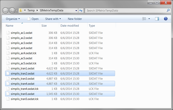
Data Settings |
File Size |
| 4000 points, no .KEEP | 4622 KB |
| 4000 points, with .KEEP | 4887 KB |
| 1634 points, with .KEEP | 1545 KB |
( not covered in class )
Change the number of plot points to 100k. Note the difference in time it takes for SIMPLIS to run the simulations. Examine the waveform fidelity with different Number of plot points.
Open the example file: 2.2_PFC_Critical_Conduction_Mode.sxsch. Run simulations and determine both the length of the vectors and the data group size on disk. Experiment with the No Forced Output Data option and compare file sizes. Compare the data file size to the Self Oscillating Converter.
© 2015 simplistechnologies.com | All Rights Reserved