Verilog-A Functions
| Name | Return type | In types | Implemented? |
| $abstime | real | () | Yes |
| $angle | real | () | No |
| $bound_step | none | (real) | Yes |
| $debug | none | ([real/integer/string...]) | Yes |
| $discontinuity | none | ([integer]) | Yes |
| $display | none | ([real/integer/string...]) | Yes |
| $fclose | none | (integer) | Yes |
| $fdebug | none | (integer, [real/integer/string...]) | Yes |
| $fdisplay | none | (integer, [real/integer/string...]) | Yes |
| $finish | none | ([integer]) | Yes |
| $fmonitor | none | (integer, [real/integer/string...]) | Yes |
| $fopen | integer | (string) | Yes |
| $fstrobe | none | (integer, [real/integer/string...]) | Yes |
| $fwrite | none | (integer, [real/integer/string...]) | Yes |
| $hflip | real | () | No |
| $limit | real | (access_func,string,real...) | No |
| $mfactor | real | () | Yes |
| $monitor | none | ([real/integer/string...]) | Yes |
| $param_given | integer | identifier | Yes |
| $port_connected | integer | identifier | Yes |
| $random | integer | (integer,[string]) | Yes |
| $rdist_chi_square | real | (integer,real, [string]) | No |
| $rdist_erlang | real | (integer,real,real, [string]) | No |
| $rdist_exponential | real | (integer,real, [string]) | No |
| $rdist_normal | real | (integer,real,real, [string]) | No |
| $rdist_poisson | real | (integer,real, [string]) | No |
| $rdist_t | real | (integer,real, [string]) | No |
| $rdist_uniform | real | (integer,real,real,[string]) | No |
| $realtime | real | ([real]) | No |
| $simparam | real | (string,[real]) | Yes |
| $stop | none | ([integer]) | Yes |
| $strobe | none | ([real/integer/string...]) | Yes |
| $table_model | real | Yes | |
| $temperature | real | () | Yes |
| $vflip | real | () | No |
| $vt | real | ([real] | Yes |
| $write | none | ([real/integer/string...]) | Yes |
| $xposition | real | () | No |
| $yposition | real | () | No |
| above | integer | (real,[real,[real]]) | No |
| abs | copies args | (real/int) | Yes |
| absdelay | real | (real, real, [real]) | Yes |
| ac_stim | complex | (string,[real,[real]]) | Yes |
| acos | real | (real) | Yes |
| acosh | real | (real) | Yes |
| analysis | integer | (string,[...]) | Yes |
| asin | real | (real) | Yes |
| asinh | real | (real) | Yes |
| atan | real | (real) | Yes |
| atan2 | real | (real,real) | Yes |
| atanh | real | (real) | Yes |
| ceil | real | (real) | Yes |
| cos | real | (real) | Yes |
| cosh | real | (real) | Yes |
| cross | integer | (real,[integer,[real,[real]]]) | Yes |
| ddt | real | (real,[real/string]) | Yes |
| ddx | real | (real,access_func) | Yes |
| exp | real | (real) | Yes |
| flicker_noise | real | (real,real,[string]) | Yes |
| floor | real | (real) | Yes |
| hypot | real | (real,real) | Yes |
| idt | real | (real,[real,[real,[real/string]]]) | Yes |
| idtmod | real | (real,[real,[real,[real,[real/string]]]]) | No |
| laplace_nd | real | (real,real-array,real-array,[real/string]) | Yes |
| laplace_np | real | (real,real-array,real-array,[real/string]) | Yes |
| laplace_zd | real | (real,real-array,real-array,[real/string]) | Yes |
| laplace_zp | real | (real,real-array,real-array,[real/string]) | Yes |
| last_crossing | real | (real,integer) | Yes |
| limexp | real | (real) | Yes |
| ln | real | (real) | Yes |
| log | real | (real) | Yes |
| max | copies args | (real/int,real/int) | Yes |
| min | copies args | (real/int,real/int) | Yes |
| noise_table | real | (real-array,[string]) | No |
| pow | real | (real,real) | Yes |
| sin | real | (real) | Yes |
| sinh | real | (real) | Yes |
| slew | real | (real,[real,[real]]) | Yes |
| sqrt | real | (real) | Yes |
| tan | real | (real) | Yes |
| tanh | real | (real) | Yes |
| timer | integer | (real,[real,[real]]) | Yes |
| transition | real | (real,[real,[real,[real,[real]]]]) | Yes |
| white_noise | real | (real,[string]) | Yes |
| zi_nd | real | (real,real-array,real-array,real,[real,[real]]) | No |
| zi_np | real | (real,real-array,real-array,real,[real,[real]]) | No |
| zi_zd | real | (real,real-array,real-array,real,[real,[real]]) | No |
| zi_zp | real | (real,real-array,real-array,real,[real,[real]]) | No |
In this topic:
$abstime
real_time = $abstime ;
In transient analysis, returns the absolute simulation time in seconds. In all other analyses returns zero.
$bound_step
$bound_step( expression ) ;
Does not return a value.
In transient analysis, instructs simulator to limit the next timestep to the value of expression.
$debug
$debug( list_of_arguments ) ;
Does not return a value.
$debug is a display function that displays information in the command shell. See $display for a description of its arguments. The $debug function writes to the command shell on every iteration. By contrast, other display functions such as $display only write information when an iteration has converged.
See Also
$discontinuity
$discontinuity [ ( constant_expression ) ] ;
Does not return a value.
Currently $discontinuity performs no action.
$display
$display( list_of_arguments ) ;
Does not return a value.
$display displays text in the command shell when the current iteration converges.
The arguments can be any sequence of strings, integers or reals. The function will display these values in the order in which they appear. The values will be output literally except for the interpretation of special characters that may appear in string values. The special characters are backslash ('\ ') and percent ('%'). '\ ' is used to output special characters according to the following table:
| \ n | Newline character |
| \ t | Tab character |
| \ \ | Literal \ character |
| \ " | " character |
| \ ddd | Character specified by the ASCII code of the 1-3 octal digits |
The '%' character must be followed by a character sequence that defines a format specification. In execution, the '%' and the format characters are substituted for the next value in the argument list, formatted according to the string. User's conversant with the 'C' programming language will have seen this method in the printf function. For example, %d specifies that an integer be displayed in decimal format. So, if count has a value of 453, the following:
$display("Count=%d", count) ;
would display:
Count=453
in the command shell.
The following table shows the format codes available:
| %h or %H | Hexadecimal format |
| %d or %D | Decimal format |
| %o or %O | Octal format |
| %b or %B | Binary format |
| %c or %C | ASCII character. E.g a value of 84 would display an uppercase 'T' |
| %m or %M | Display hierarchical name of instance. This does not use one of the subsequent arguments |
| %s or %S | Literal string. Expects a matching string argument |
| %e or %E | Real number format. See Real Number Formats below |
| %f or %F | Real number format. See Real Number Formats below |
| %g or %G | Real number format. See Real Number Formats below |
| %r or %R | Real number format. See Real Number Formats below |
Real Number Formats
Real numbers have their own more complex format codes. These are in the form:
% [flag] [width] [.precision] type
where:
| flag | Characters '-', '+', '0', space or '#'. '-' means left align the result within given width (see width) '+' means always prefix a sign even if positive '0' means prefix with leading zeros '#' forces a decimal point to be always output even if not required |
| width | Specifies the minimum number of characters that will be displayed, padding with spaces or zeros if needed |
| precision | For e and f formats (see below) specifies the number of digits after the decimal point that will be printed. If g or r format is specified, specifies the maximum number of significant digits. Default if omitted is 6. |
| type | e, E, f, F, g, G or r, R e or E: Signed value displayed in exponential format. E.g. 1.23456E3 f or F: Signed value in decimal format. E.g. 1234.56. Result will be very long if value is very large or very small. g or G: Uses either f or e depending on which is most compact for give precision. r or R: displays in engineering units. Uses these scale factors: T, G, M, K, k, m, u, n, p, f, a. |
Notes
integer count ;
...
$display("Count=%g", count) ;
Note that the type (i.e. integer or real) of literal constants is determined by the way they are written. If a decimal point is included or if exponential or engineering formats are used, the number is real. Otherwise it is an integer. So '11' is an integer, while 11.0 is a real.
See Also
$fclose
$fclose( file_descriptor ) ;
Does not return a value.
Closes one or more file descriptors opened with $fopen.
See Also
$fdebug
$fdebug( file_descriptor, list_of_arguments ) ;
Does not return a value.
As $debug, but writes to a file or files defined by file_descriptor.
See Also
$fdisplay
$fdisplay( file_descriptor, list_of_arguments ) ;
Does not return a value.
As $display, but writes to a file or files defined by file_descriptor.
See Also
$finish
$finish [ ( n ) ]
Does not return a value.
Instructs simulator to abort. Currently the argument is ignored.
$fmonitor
$fmonitor( file_descriptor, list_of_arguments ) ;
Does not return a value.
As $monitor, but writes to a file or files defined by file_descriptor.
$fopen
integer file_descriptor = $fopen( filename ) ;
Returns an integer representing a multi-channel file descriptor. The descriptor can be used as an argument to $fdebug, $fdisplay, $fmonitor, $fstrobe and $fwrite to write output to a file.
There are 31 possible channels each represented by a single bit in the 32 bit returned value. The top (most significant bit) is reserved. The bottom (least siginificant) is used for standard output - i.e. displays to the command shell. Each new call to $fopen will assign the next channel and set the relevant bit. By or'ing together the results from multiple calls to $fopen, it is possible to write to more than one file at a time.
SIMetrix has a special extension to this function providing access to the list file. Use the filename "<listfile>" and the descriptor returned will access it. The following code for example will create a file descriptor that will provide writes to both the list file and a user file:
fd = $fopen( "<listfile>" ) ;
fd = fd | $fopen( "a_text_file.txt") ;
Further, by or'ing with 1 the file descriptor will also write to the command shell.
The file descriptor should be closed with $fclose.
See Also
$fstrobe
$fstrobe( file_descriptor, list_of_arguments ) ;
Does not return a value.
As $strobe, but writes to a file or files defined by file_descriptor. Note that the $strobe and $display functions are identical. For detailed documentation see $display.
See Also
$fwrite
$fwrite( file_descriptor, list_of_arguments ) ;
Does not return a value.
As $write, but writes to a file or files defined by file_descriptor. Note that the $write function is identical to $display, except that it does add a new line character. For detailed documentation see $display.
See Also
$mfactor
real_value = $mfactor ;
$mfactor does not take any arguments.
Returns the scaling factor applied to the instance. The scaling factor may be set using the $mfactor parameter or using a subcircuit multiplier M. If both are used, the final scale factor will be the product of these. Refer to the LRM for more details.
The LRM currently stipulates that compilers should raise an error if $mfactor is used inappropriately. This is not currently implemented and $mfactor may be used for any purpose.
$monitor
$monitor( list_of_arguments ) ;
Does not return a value.
$monitor behaves in a similar manner to $display except that it only outputs a result when there is a change. In other words, the behaviour is the same as $display except that successive repeated messages will not be output.
See Also
$param_given
integer_value = $param_given( parameter_name ) ;
parameter_name must be a parameter defined using the parameter keyword. Returns a non-zero number if parameter_name has been specified in a .MODEL statement or on the instance line where relevant.
$port_connected
integer_value = $port_connected( port_name[ [index_expression] ] ) ;
Returns a non-zero value if the specified port_name is connected externally. If the port is vectored, then index_expression defining the element within the vector must also be specified. No error will be raised if the index supplied is out of range; the function will simply return false (zero).
Currently, this function will only deem a port to be unconnected if no node is specified for it in the instance netlist line. It will return true (non-zero) if a node name is supplied on the netlist line but is not connected to any other component in the netlist. For example, consider a model for a four-terminal BJTwith nodes 'C', 'B', 'E' and 'S' where 'S' is the substrate connection:
Q1 C B E S bjtmodelname
In the above the substrate connection is the node S. In this case $port_connected(S) would return true regardless of whether or not S was connected to anything else. Now consider the three terminal case:
Q1 C B E bjtmodelnameIn this case the substrate connection has been omitted from the netlist line and $port_connected will return false (zero).
$random
integer_value = $random [ (seed) ] ;
Returns a random number. This has three modes of operation according what if anything is supplied for seed.
Mode 1: no seed
$random will return a new random number on each call with the system choosing the seed when random is used for the first time.
Example:
value = $random ;
Mode 2: constant seed
seed may be either a literal constant or a constant expression dependent only on literal constants and parameters. In this mode $random will return a fixed random value which will not update.
Example:
parameter seed=23 ;
...
value = $random(seed) ;
Mode 3: initialised integer variable seed
In this mode the seed variable will be updated on each call and a new random number will be generated. The sequence of random numbers will thus be repeatable given the same initial value for seed.
Example:
real seed ;
...
@(initial_step)
seed = 23 ;
...
value = $random(seed) ;
In the above, the value of seed will be updated each time random is called.
$simparam
real_value = $simparam( string [ , default_value ] ) ;
Returns the value of a simulator parameter defined by string. Possible values of string are described below. If an unknown string is supplied, $simparam will return the value of default_value if given. If no default_value value is given, a run-time error will be raised.
| "gdev" | Conductance added in junction GMIN stepping algorithm |
| "gmin" | Value of GMIN options parameter |
| "simulatorSubversion" | Minor version of SIMetrix simulator. E.g. for version 6.00, result will be 0, for 6.10 result will be 10 etc |
| "simulatorVersion" | Major version of SIMetrix simulator. For version 6.00 this will be 6 |
| "sourceScaleFactor" | Scale factor used for sources in source stepping algorithm and pseudo transient analysis algorithm |
| "tnom" | Value of TNOM options parameter |
| "ptaScaleFactor" | Scale factor used for pseudo transient analysis algorithm |
| "option_name" | Any name that may be used in a .OPTIONS statement and which has a real value |
The first six items in the above follow recommended names in the Verilog-A LRM. The remainder are special to SIMetrix.
$stop
$stop [ ( n ) ] ;
The function does not return a value. Pauses simulation after completion of current step and leaves the simulator in the same state as if the user pressed the pause button.
The argument n currently has no effect.
See Also
$strobe
$strobe( list_of_arguments ) ;
Does not return a value.
Identical to the $display function.
See Also
$table_model
real_value =
$table_model( table_inputs, table_data_source, table_control_string) ;
Please refer to section 10.12 of the Verilog-AMS Language Reference Manual version 2.2. This can be obtained from http://www.eda.org/verilog-ams/htmlpages/lit.html. SIMetrix implements the LRM specification in full.
$table_model is subject to the same restrictions as analog operators according to the Verilog-A version 2.2 LRM (See Analog Operator Restrictions). This restriction has been removed from the version 2.3 standard and indeed there is no fundamental reason for the restriction as the $table_model function does not need to store state information. Currently, SIMetrix complies with LRM 2.2 - i.e the restrictions apply - but we plan to change this with a future release.
$temperature
real_value = $temperature ;
Returns the current simulation temperature in Kelvin.
$vt
real_value = $vt [ ( temperature_expression ) ] ;
Returns the thermal voltage at temperature_expression. If temperature_expression is not supplied, the value at the current simulation temperature will be returned.
The thermal voltage is defined as
\[ \frac{KT}{q} \]
Where, ???MATH???K???MATH??? is boltzmann's constant, ???MATH???T???MATH??? is temperature (defined by temperature_expression) and ???MATH???q???MATH??? is the charge on an electron. The values used for ???MATH???K???MATH??? and ???MATH???q???MATH??? are those that are used for other simulator models and are the best values known at the time the original SPICE program was developed. Since that time the accepted values for ???MATH???K???MATH??? and ???MATH???q???MATH??? have been altered slightly.
- ???MATH???K = 1.3806226\text{e-23}???MATH???
- ???MATH???q = 1.6021918\text{e-19}???MATH???
- ???MATH???K = 1.3806504\text{e-23}???MATH???
- ???MATH???q = 1.60217646\text{e-19}???MATH???
$write
$write( list_of_arguments ) ;
Does not return a value.
$write is identical to the $display function except that it does not add a new line character at the end of the text. A new line may be explicitly inserted using the '\ n' sequence.
See Also
abs
real_value = abs( x ) ;
Returns the absolute value of x.
absdelay
real_value = absdelay( expression, tdelay [ , maxdelay ] ) ;
Applies a transport delay to an input signal.
| expression | Input signal to delay. |
| tdelay | Delay in seconds. If maxdelay is not supplied, only the value of tdelay at the start of the simulation will be used and subsequent changes will be ignored. Otherwise changes to tdelay will be used as long as they do not exceed maxdelay. |
| maxdelay | Maximum delay permitted. If omitted changes to tdelay will be ignored. See tdelay above. |
In DC analyses, tdelay is ignored and the return value of absdelay is expression. In AC analysis, the signal defined by expression is phase-shifted according to:
\[ \text{output}\left(\omega\right) = \text{input}\left(\omega\right)\exp(-j\omega\cdot\text{tdelay}) \]
In transient analysis, the signal is delayed by an amount equal to the instantaneous value of tdelay as long as it is positive and less than maxdelay. absdelay stores the past history of expression up to maxdelay so that it can retrieve the requested delayed point instantaneously.
absdelay is an analog operator and is subject to Analog Operator Restrictions.
See Also
ac_stim
real_value = ac_stim( [analysis_name_string [ , mag [ , phase ]]] ) ;
Provides a stimulus for AC analysis, essentially identical the AC spec for a standard SPICE voltage source or current source.
| analysis_name_string | Analysis name in which source is to be active. Currently this must be set to "ac" or be omitted altogether. |
| mag | Magnitude of source |
| phase | Phase of source in radians |
acos
real_value = acos( x ) ;
Returns inverse cosine in radians of x. Input range is +/- 1.
acosh
real_value = acosh( x ) ;
Returns the inverse hyperbolic cosine of x. Range is 1.0 to ???MATH???\infty???MATH???.
analysis
integer_value = analysis( analysis_list ) ;
Returns non-zero if the current analysis matches any of the analysis names in the argument list. analysis_list is a list of strings as defined in the following table.
| "static" | Any analysis that solves a DC operating point. This includes the operating point analyses carried before other analyses such as transient. It also includes DC sweep |
| "tran" | Transient analysis. Includes the transient analysis used for pseudo transient analysis |
| "ac" | AC analysis |
| "dc" | DC sweep |
| "noise" | Noise analysis not including real time noise |
| "tf" | Transfer fumction analysis |
| "pz" | Pole zero analysis |
| "sens" | Sensitivity analysis |
| "ic" | The dc operating point analysis that precedes a transient analysis |
| "smallsig" | Any small signal analysis: AC, noise and TF |
| "rtn" | Real-time noise analysis |
| "pta" | Pseudo transient analysis |
asin
real_value = asin (x ) ;
Returns the inverse sine in radians of x. Range is +/- 1.0.
asinh
real_value = asinh( x ) ;
Returns the inverse hyperbolic sine of x. Range is ???MATH???-\infty???MATH??? to ???MATH???+\infty???MATH???.
atan
real_value = atan( x ) ;
Returns the inverse tangent in radians of x. Range is ???MATH???-\infty???MATH??? to ???MATH???+\infty???MATH???.
atan2
real_value = atan2( x, y ) ;
Returns the inverse tangent in radians of x/y. The function will return a meaningful value when y is zero.
atanh
real_value = atanh( x ) ;
Returns the inverse hyperbolic tangent of x. Range is +/- 1.0.
ceil
real_value = ceil( x ) ;
Returns the next integer value greater than x.
See Also
cos
real_value = cos( x ) ;
Returns the cosine of x expressed in radians. Range is ???MATH???-\infty???MATH??? to ???MATH???+\infty???MATH???.
cosh
real_value = cosh( x ) ;
Returns the hyperbolic cosine of x. Range is approx -709 to +709.
cross
cross( expression [,edge [,time_tol [,expr_tol ]]])
cross is an event function and may only be used in event expressions.
| expression | expression to test. The event is triggered when the expression crosses zero. |
| edge | 0, +1 or -1 to indicate edge. +1 means the event will only occur when expr is rising, -1 means it will only occur while falling and 0 means it will occur on either edge. Default=0 if omitted. |
| time_tol | Time tolerance for detection of zero crossing. Unless the input is moving in an exact linear fashion, it is not possible for the simulator to predict the precise location of the crossing point. But it can make an estimate and then cut or extend the time step to hit it within a defined tolerance. time_tol defines the time tolerance for this estimate. The event will be triggered when the difference between the current time step and the estimated crossing point is less than time_tol. If omitted or zero or negative, no timestep control will be applied and the event will be triggered at the first natural time point after the crossing point. See diagram below for an illustration of the meaning of this parameter. |
| expr_tol | Similar to time_tol but instead defines the tolerance on the input expression. See figure below. |
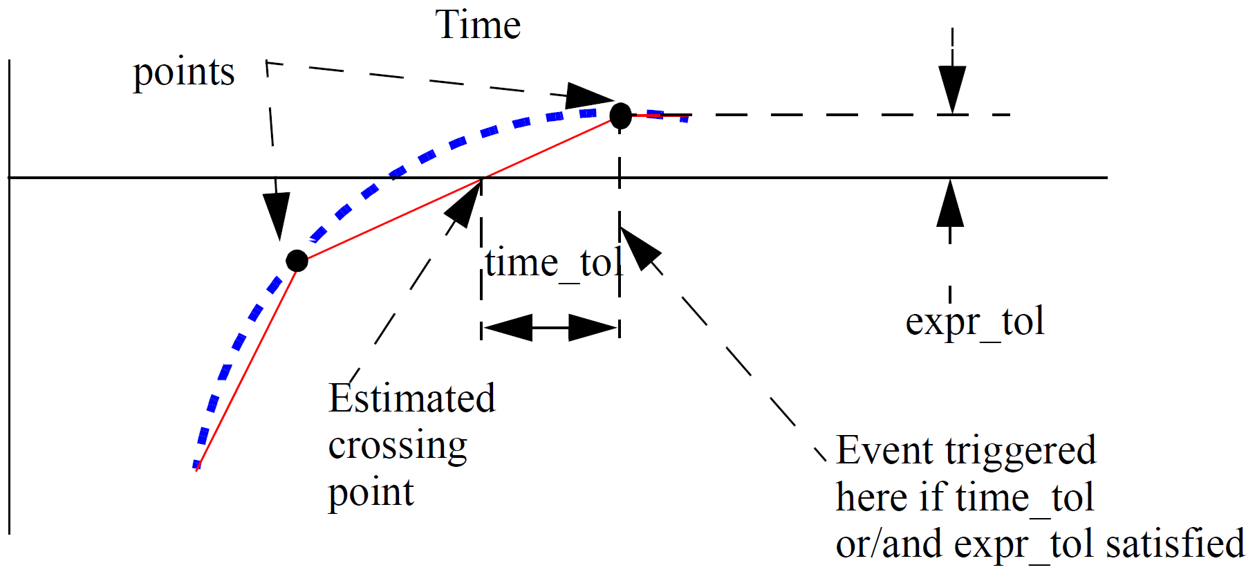 |
Cross Event Function Behaviour |
cross stores state information in the same way as an analog operator. It is therefore subject to Analog Operator Restrictions.
See Also
ddt
real_value = ddt( expression ) ;
Returns the time derivative of expression:
\[ \frac{d}{dt}\text{expression} \]
In DC analyses, ddt returns zero. In AC analysis, the function is defined by the relation:
\[ \text{output}\left(\omega\right) = input\left(\omega\right)\cdot j\omega \]
ddt is an analog operator and is subject to Analog Operator Restrictions.
See Also
ddx
real_value = ddx( expression, unknown_variable) ;
Performs symbolic differentiation on expression with respect to unknown_variable, which must be defined in terms of an access function in one of the following forms:
potential_access_identifier( net_or_port_scalar_expression )OR
flow_access_identifer( branch_identifier )
A potential_access_identifier is defined in the discipline declarations and is usually 'V' for the electrical discipline. Similarly, the flow_access_identifier is usually 'I' for the electrical discipline.
net_or_port_scalar_expression can be a module port node or an internal node.
branch_identifier can be a branch defined with the branch keyword or an unnamed branch specifying the nodes connected to the branch.
exp
real_value = exp( x ) ;
Returns the exponential of x. Range is ???MATH???-\infty???MATH??? to about 709.
See Also
flicker_noise
real_value = flicker_noise( power, exp [, name]) ;
flicker_noise is only active in small-signal noise analysis and real-time noise analysis; in other analysis modes it returns zero. It creates a noisy signal with a power of power at 1Hz which varies in proportion to ???MATH???1/f^{\text{exp}}???MATH???.
name may be used to combine noise sources in the output report and vectors. Noise sources with the same name in the same instance will be combined together.
In real-time noise analysis flicker_noise simply returns a random number whose statistical distribution satisfies the characteistic of ???MATH???1/f???MATH??? noise. In small signal analysis flicker_noise defines a ???MATH???1/f???MATH??? noise source that may be propagated to any output node.
See Also
hypot
real_value = hypot( x, y ) ;
Returns ???MATH???\sqrt{x^2 + y^2}???MATH???.
idt
real_value = idt( expression [, initial_condition ] ) ;
Returns the time integral of expression.
initial_condition if supplied, sets the value of the function for DC analyses including the dc operating point that precedes other analyses.
If initial_condition is not supplied, idt must exist inside a closed feedback loop. With no initial condition the DC gain of idt is infinite; by putting the function inside a loop, the simulator can maintain the input at zero providing a finite output. A singular matrix error will result otherwise.
idt is an analog operator and is subject to Analog Operator Restrictions.
See Also
laplace_nd
real_value = laplace_nd(expr, num_coeffs, den_coeffs [, $\epsilon$]) ;
| expr | Input expression. |
| num_coeffs | Numerator coefficients. This can be entered as an array variable or as an array initialiser. An array initialiser is a sequence of comma separated values enclosed with '{' and '}'. E.g: { 1.0, 2.3, 3.4, 4.5}. The values do not need to be constants. |
| den_coeffs | Denominator coefficients in the same format as the numerator - see above. |
| ???MATH???\epsilon???MATH??? | Tolerance parameter currently unused. |
The laplace_nd analog operator implements a Laplace transfer function. This is in the form:
\[ H(s) = \frac{n_0 + n_1\cdot s + n_s\cdot s^2 + ... + n_m\cdot s^m}{d_0 + d_1\cdot s + d_2\cdot s^2 + ... + d_m\cdot s^m} \]
where ???MATH???d_0, d_1, d_2, ..., dm???MATH??? are the denominator coefficients and ???MATH???n_0, n_1, n_2, ..., n_m???MATH??? are the numerator coefficients and the order is ???MATH???m???MATH???.
If the constant term on the denominator ( ???MATH???d_0???MATH??? in equation above) is zero, the laplace function must exist inside a closed feedback loop. With a zero denominator, the DC gain is infinite; by putting the function inside a loop, the simulator can maintain the input at zero providing a finite output. A singular matrix error will result otherwise.
laplace_nd is an analog operator and is subject to Analog Operator Restrictions.
See Also
laplace_np
real_value = laplace_np(expr, num_coeffs, poles [, $\epsilon$]) ;
| expr | Input expression |
| zeros | Zeros. See laplace_zp for details. |
| den_coeffs | Denominator coefficients. See laplace_nd for details. |
| ???MATH???\epsilon???MATH??? | Tolerance parameter currently unused |
laplace_np is an analog operator and is subject to Analog Operator Restrictions.
See Also
laplace_zd
real_value = laplace_zd(expr, zeros, den_coeffs [, $\epsilon$]) ;
| expr | Input expression. |
| zeros | Zeros. See laplace_zp for details. |
| den_coeffs | Denominator coefficients. See laplace_nd for details. |
| ???MATH???\epsilon???MATH??? | Tolerance parameter currently unused. |
laplace_zd is an analog operator and is subject to Analog Operator Restrictions.
See Also
laplace_zp
real_value = laplace_zp(expr, zeros, poles [, $\epsilon$]) ;
| expr | Input expression. |
| zeros | Array of pairs of real numbers representing the zeros of the Laplace transform. Each pair consists of a real part and an imaginary part with the real part first. Each zero introduces a product term on the numerator in the form: \[ 1-\frac{s}{\textit{re} + j\cdot \textit{im}} \] where re is the real part and im imaginary part. If a zero is complex (i.e. the imaginary part is non-zero) then its complex conjugate must also be present. If both real and imaginary parts are zero then the zero becomes just s. The values can be entered as an array variable or as an array initialiser. An array initialiser is a sequence of comma separated values enclosed with '{' and '}'. E.g: {1.0, 2.3, 3.4, 4.5}. The values do not need to be constants. |
| poles | Array of pairs of real numbers representing the poles of the Laplace transform. Each pair consists of a real part and an imaginary part with the real part first. Each pole introduces a product term on the denominatr in the form: \[ 1-\frac{s}{\textit{re} + j\cdot \textit{im}} \] where re is the real part and im imaginary part. If a pole is complex (i.e. the imaginary part is non-zero) then its conjugate must also be present. If both real and imaginary parts are zero then the pole becomes just s. The values can be entered as an array variable or as an array initialiser. An array initialiser is a sequence of comma separated values enclosed with '{' and '}'. E.g: {1.0, 2.3, 3.4, 4.5}. The values do not need to be constants. |
| ???MATH???\epsilon???MATH??? | Tolerance parameter currently unused. |
laplace_zp is an analog operator and is subject to Analog Operator Restrictions.
See Also
last_crossing
real_value = last_crossing( expression, direction ) ;
last_crossing returns the time in seconds when expression last crossed zero. First order interpolation is used to estimate the time of the crossing. direction controls the direction of the crossing. If +1 then the most recent positive transition is returned. If -1, the most recent negative transition and if zero the most recent in either direction is returned.
last_crossing returns a negative number if expression has not crossed zero since the start of the simulation. SIMetrix Verilog-A last_crossing implementation also returns a negative number for DC analyses but this is not defined in the standard.
last_crossing is an analog operator and is subject to Analog Operator Restrictions.
limexp
real_value = limexp( x ) ;
Returns the exponential of x. limexp limits its change in output from iteration to iteration in order to improve convergence. In situations where its return value is not the true exponential of x it will force further iterations. The iteration will only be accepted when the result is the true value of exp(x). Thus, limexp can be seen as a direct replacement for exp but with improved convergence. But note that limexp is an analog operator and is therefore subject to Analog Operator Restrictions.
See Also
ln
real_value = ln( x ) ;
Returns the natural logarithm of x. Range is 0.0 to ???MATH???\infty???MATH???.
log
real_value = log( x ) ;
Returns the logarithm to base 10 of x. Range is 0.0 to ???MATH???\infty???MATH???.
max
real_value = max( x, y ) ;
Returns x or y whichever is larger. Equivalent to ( x>y ? x : y )
min
real_value = min( x, y ) ;
Returns x or y whichever is smaller. Equivalent to ( x<y ? x : y )
pow
real_value = pow( x, y ) ;
Returns ???MATH???x^y???MATH???. if x is less than zero, y must be an integer. If ???MATH???x=0???MATH???, y must be greater than zero.
sin
real_value = sin( x ) ;
Returns the sine of x given in radians. Range ???MATH???-\infty???MATH??? to ???MATH???\infty???MATH???.
sinh
real_value = sinh( x ) ;
Returns the hyperbolic sine of x. Range is approx -709 to +709.
slew
real_value = slew( expression [, slew_pos [, slew_neg]] ) ;
Implements a slew rate limiter. slew_pos is expected to be positive and slew_neg is expected to be negative. If slew_neg is not specified or greater than or equal to zero, it assumes a value of -slew_pos. If neither slew_pos or slew_neg is present, expression is passed through to value unchanged.
slew limits the positive and negative rate of change of its return value to slew_pos and slew_neg respectively.
slew is an analog operator and is subject to Analog Operator Restrictions.
See Also
sqrt
real_value = sqrt( x ) ;
Returns the square root of x. Range is 0 to ???MATH???\infty???MATH???. Although valid, ???MATH???x=0???MATH??? should be avoided and if possible code included to prevent ???MATH???x=0???MATH???. This is because the first derivative of sqrt at zero is infinite and convergence at this value can be problematic.
tan
real_value = tan( x ) ;
Returns the tangent of x given in radians. Range is ???MATH???-\infty???MATH??? to ???MATH???\infty???MATH???.
tanh
real_value = tanh( x ) ;
Returns the hyperbolic tangent of x. Range is ???MATH???-\infty???MATH??? to ???MATH???\infty???MATH???.
timer
timer( time [, period [, time_tol]])
timer is an event function and may only be used in an event statement in the form:
@(timer(...))
statement ;
statement is executed when the event is triggered.
timer sets a future event to occur at a specified time either just once or repeating at a specified period.
The event is first scheduled at time. If period is specified and is greater then zero, subsequent events will also be scheduled at time + n*period where n is a positive integer.
Usually the specified event will be scheduled at exactly the time specified. However, the analog simulator will not allow time points to be forced too close together as this can lead to numerical problems as well as unnecessarily long simulation times. For this reason, the simulator may schedule the event slightly later than specified if the time point is to close to an existing time point, perhaps set by another device. The time_tol argument controls the tolerance of the event time. The simulator will always schedule the event so that it is within time_tol of the requested time. If time_tol is not specified the event will be scheduled after the requested time but not more than the amount specified by the MINBREAK simulaion parameter.
See Also
transition
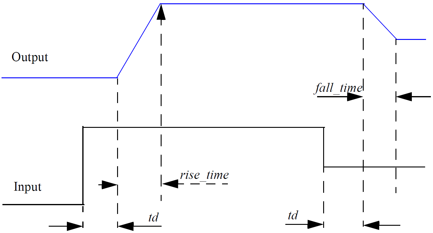
real_value = transition(expr[, td[, rise_time[, fall_time [, time_tol]]]]);
The transition analog operator converts the discrete input value to a continuous output value using specified rise and fall times.
Its arguments are:
| expr | Input expression. |
| td | Delay time. This is a transport or stored delay. That is, all changes will be faithfully reproduced at the output after the specified delay time, even if the input changes more than once during the delay period. This is in contrast to inertial delay which swallows activity that has a shorter duration than the delay. Default=0. |
| rise_time | Rise time of output in response to change in input. |
| fall_time | Fall time of output in response to change in input. |
| time_tol | Currently ignored. |
If fall_time is omitted and rise_time is specified, the fall_time will default to rise_time. If neither is specified or are set to zero, a minimum but non-zero time rise/fall time is used. This is set to the value of MINBREAK which is the minimum break point value. Refer .OPTIONS in the Simulator Reference Manual/Command Reference/.OPTIONS for details of MINBREAK.
The transition analog operator should not be used for continuously changing input values; use the slew or absdelay analog operators instead.
transition is an analog operator and is subject to Analog Operator Restrictions.
See Also
white_noise
real_value = white_noise( power [, name]) ;
white_noise is only active in small-signal noise analysis and real-time noise analysis; in other analysis modes it returns zero. It creates a noisy signal with a power of power and a flat frequency distribution.
name may be used to combine noise sources in the output report and vectors for small-signal noise analysis. name is ignored with real-time noise analysis. Noise sources with the same name in the same instance will be combined together.
In real-time noise analysis white_noise simply returns a random number whose statistical distribution satisfies the characteistic of Gaussian noise. In small signal analysis white_noise defines a noise source that may be propagated to any output node.
See Also
| ◄ Verilog-A Reference | Analog Operator Restrictions ▶ |