Example of Applying the POP Analysis Tool

The regulated converter in Example 5 of Chapter 9 is used here as an example in applying the periodic operating point analysis tool. The schematic associated with this example is repeated here in fig 10.7. In particular, we would like to examine the transient response of this regulated converter when the input voltage VI is abruptly changed from 40V to 30V, with the load RL fixed at 10. The variables of interest are the output voltage V(RL) and the current I(L) through the filter inductor. The input file describing this analysis is shown in fig 10.8 . To make the transient response more pronounced, some of the component values have been changed from those listed in Example 5 of Chapter 9. In particular, the values on C1, C14, and R14 have been changed to 0.005 F, 10 pF, and 40 k, respectively.

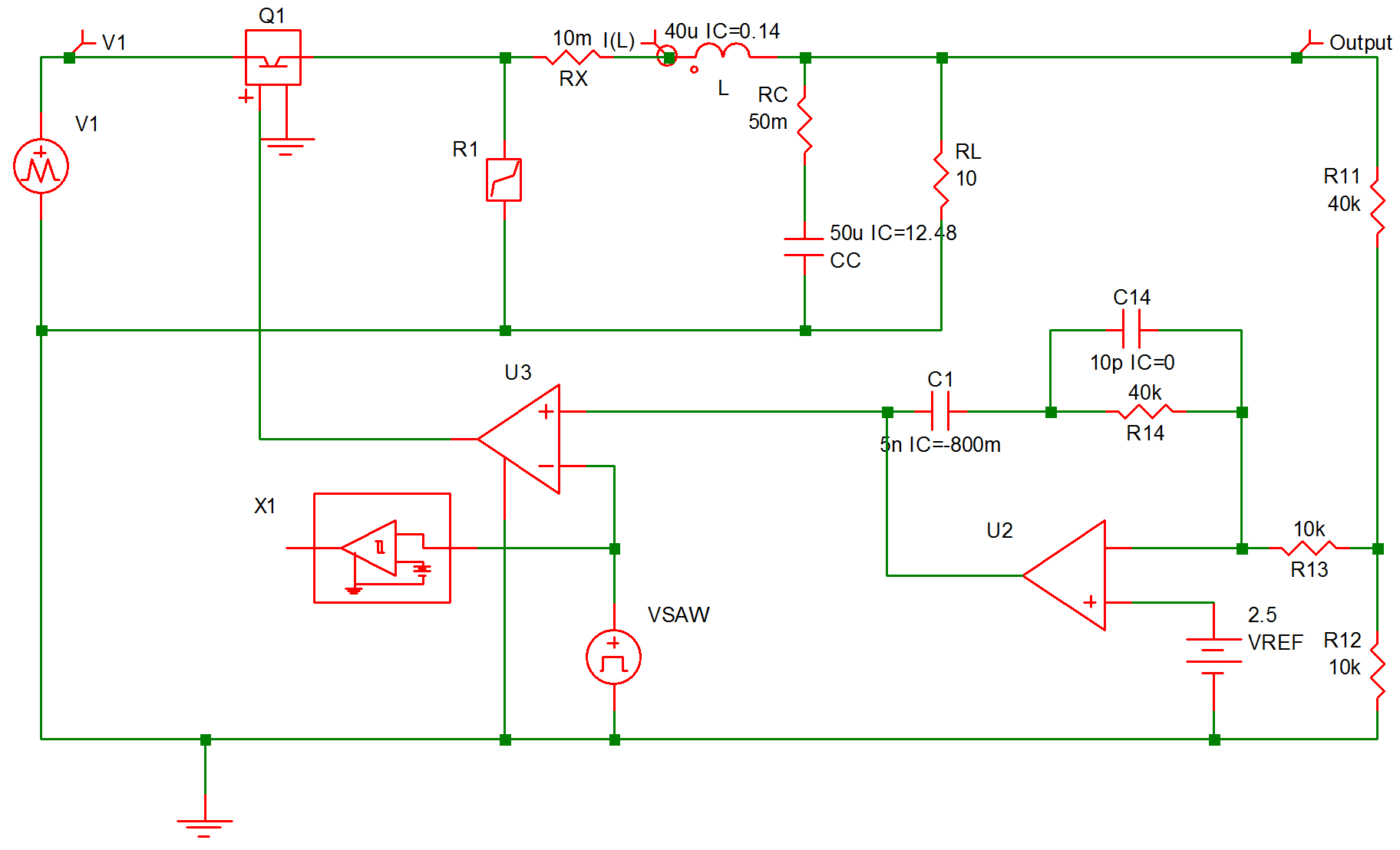10.7 Regulated Converter

*pop-example.sxsch
.PRINT  ALL
.OPTIONS  PSP_NPT=2001  POP_ITRMAX=40
.POP  TRIG_GATE=X1.!D_CYCLE  TRIG_COND=1_TO_0  MAX_PERIOD=50u
.TRAN 2m 0
X$U2 11 14 10 opamp
VSAW 12 0 SAW V1=0 V2=5 FREQ=100k DELAY=0 OFF_UNTIL_DELAY=NO
X$U3 6 0 11 12 SIMPLIS_COMP$1
V1 2 0 PWL NSEG=3 X0=0 Y0=40 X1=100U Y1=40 X2=100U Y2=30
+ X3=100M Y3=30
VREF 14 0 2.5
L 4 5 40u IC=0.14
R12 0 8 10k
X1 12 13 PERIODIC_OP$2
R13 8 10 10k
RC 7 5 50m
RL 5 0 10
R11 8 5 40k
C1 11 9 5n IC=-800m
R14 10 9 40k
C14 9 10 10p IC=0
CC 7 0 50u IC=12.48
Q1 2 3 6 0 Q1$TP_VCQ IC=OPEN
.MODEL Q1$TP_VCQ VCQPOS VSAT=700m RSAT=100m ROFF=10Meg GAIN=10
+ TH=2.5 HYSTWD=1u LOGIC=POS LEVEL=1
!R$R1 0 3 R1$TP_SSPWLR IC=1
.MODEL R1$TP_SSPWLR VPWLR NSEG=2 X0=0 Y0=0 X1=0.7 Y1=10U
+ X2=0.8 Y2=1.00001
RX 4 3 10m
.SUBCKT PERIODIC_OP$2  1 3
.NODE_MAP IN 1
.NODE_MAP OUT 3
!D_CYCLE 3 0 1 302 M1M IC=0
VREF 302 0 DC 2.5
.MODEL M1M COMP RIN=10MEG ROUT=50 VOL=0 VOH=5
+ HYSTWD=0.001 DELAY=0
.ENDS PERIODIC_OP$2
.SUBCKT SIMPLIS_COMP$1  201 100 101 102
!DCOMP 201 100 101 102 MCOMP IC=1
.MODEL MCOMP COMP RIN=1e+007 ROUT=50 VOL=0 VOH=5
+ HYSTWD=0.001 DELAY=0
.ENDS SIMPLIS_COMP$1
.SUBCKT opamp  2 3 1
.NODE_MAP VINN 1
.NODE_MAP VINP 3
.NODE_MAP VOUT 2
RIN 3 1 5Meg
EOP 2 0 3 1 1Meg
.ENDS opamp
.END

To obtain the transient response in this study, a time-domain transient simulation with the voltage of VI set at 30V is carried out after a periodic operating point analysis is applied to the system with the voltage of VI set at 40V. Notice that the initial conditions defined for the various components from Example 5 in Chapter 9 correspond to the steady-state operating conditions when the voltage of VI is at 40V. Obviously, if one already knows the steady-state solution, there is no point in running a POP analysis to find the steady-state solution. For the purpose of illustration, the initial conditions in the input file shown in Figure 10-8 have been changed, providing SIMPLIS with initial information which is not within the immediate vicinity of the steady-state solution.

The input voltage source VI is now modeled as a piecewise-linear source instead of a DC source. Its source value jumps from 40V to 30V when t = 100 s. To find the steady-state solution of the system when the voltage of VI is 40V, the periodic operating analysis tool is invoked by using the .POP statement as shown. The comparator !D$U3 defines the start of a switching cycle as the moment when the value of the sawtooth source VSAW is decreasing and reaching the value of approximately 2.5V. Since the source VI is a piecewise-linear source, its source value is held constant at 40V, its initial value, during the POP analysis. As a result, the steady-state solution as computed by the periodic operating analysis tool corresponds to the steady-state solution of the system when VI is at 40V.

After the POP analysis is finished, SIMPLIS carries out a regular time-domain transient simulation according to the .TRAN statement for 2000s. As explained in How POP Deals with Time Varying Sources, the source value of VI will be at 40V for the first 100s in this transient simulation and at 30V for the rest of the simulation. Waveforms as obtained in this time-domain transient analysis for V(VI), V(RL), and I(L) are shown in fig 10.9 .

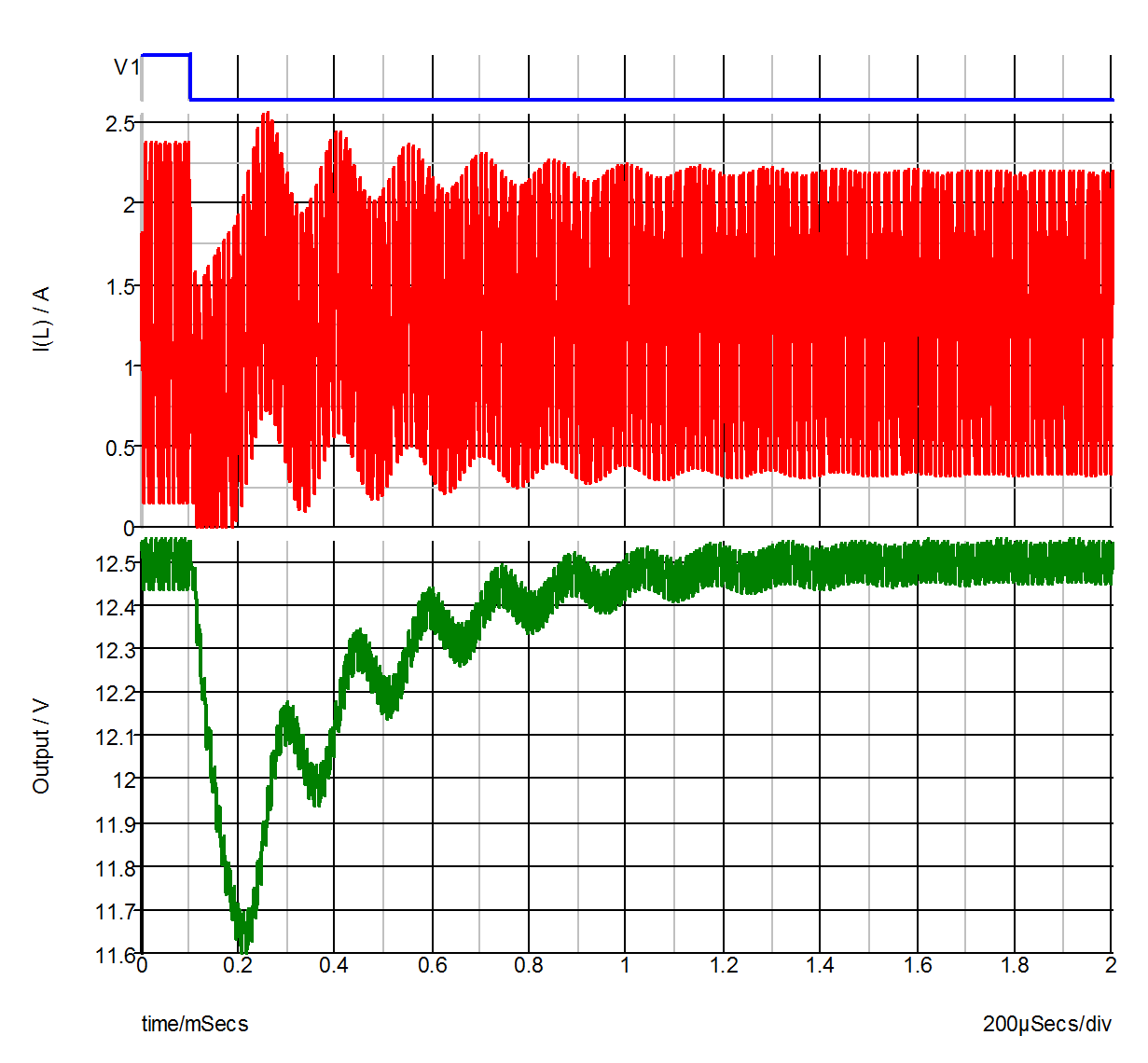10.9 Waveforms obtained in time-domain analysis for V(VI), V(RL), and I(L).