Laplace Transfer Function - Lumped Implementation
In this topic:
Netlist entry
Axxxx input output model_name
Connection details
| Name | Description | Flow | Default type | Allowed types |
| in | Input | in | v | v, vd, i, id |
| out | Output | out | v | v, vd, i, id |
Model format
.MODEL model_name s_xfer parameters
Model parameters
| Name | Description | Type | Default | Limits | Vector bounds |
| in_offset | Input offset | real | 0 | none | n/a |
| gain | Gain | real | 1 | none | n/a |
| laplace | Laplace expression (overrides num_coeff and den_coeff) | string | none | none | n/a |
| num_coeff | Numerator polynomial coefficient | real vector | none | none | ???MATH???1 - \infty???MATH??? |
| den_coeff | Denominator polynomial coefficient | real vector | none | none | ???MATH???1 - \infty???MATH??? |
| int_ic | Integrator stage initial conditions | real vector | 0 | none | none |
| denormalized_freq | Frequency (radians/second) at which to denormalize coefficients | real | 1 | none | n/a |
Description
This device was formerly known as the S-domain Transfer Function Block. It implements an arbitrary linear transfer function expressed in the frequency domain using a Laplace transform. This is one of two models that can implement a Laplace transfer function. The other one is Laplace Transfer Function Convolution Implementation
The operation and specification of the device is illustrated with the following examples.
Examples
Example 1 - A single pole filter
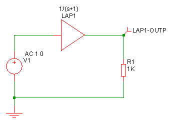
Model for above device:
.model Laplace s_xfer laplace="1/(s+1)" denormalized_freq=1
This is a simple first order roll off with a 1 second time constant as shown below
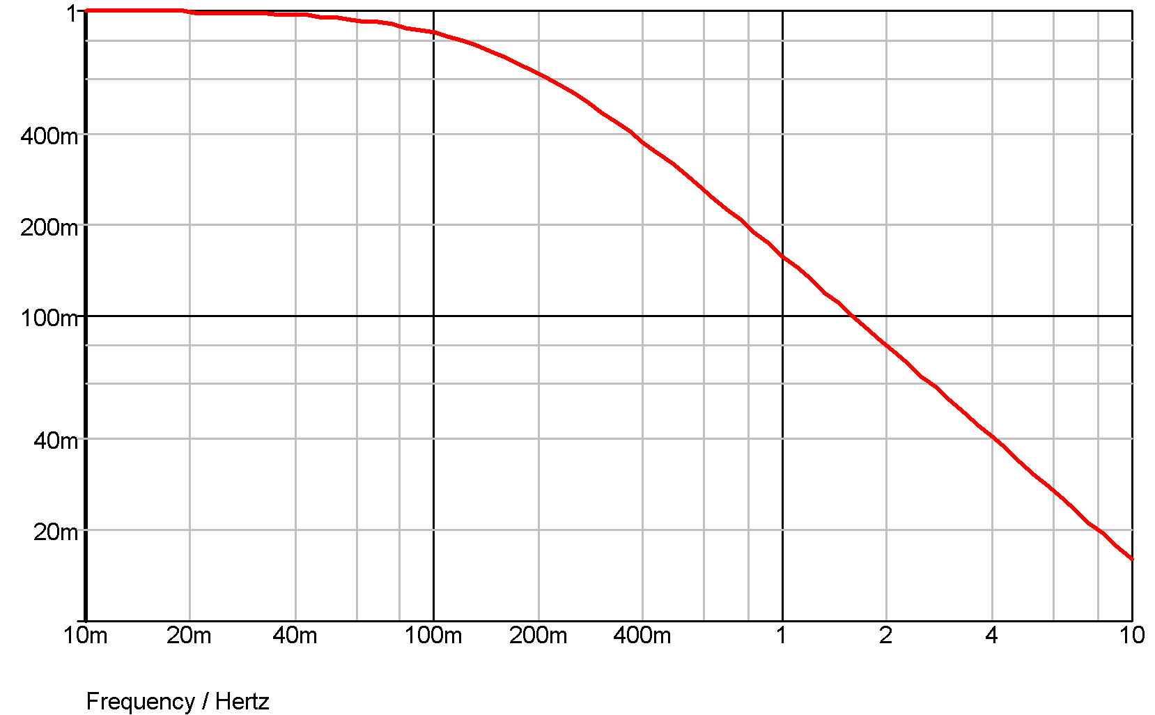
Example 2 - Single pole and zero
.model Laplace s_xfer
+ laplace="(1/s)/(1/s + 1/(0.1*s+1))"
+ denormalized_freq=1
The laplace expression has been entered how it might have been written down without any attempt to simplify it. The above actually simplifies to (0.1*s+1)/(1.1*s+1).
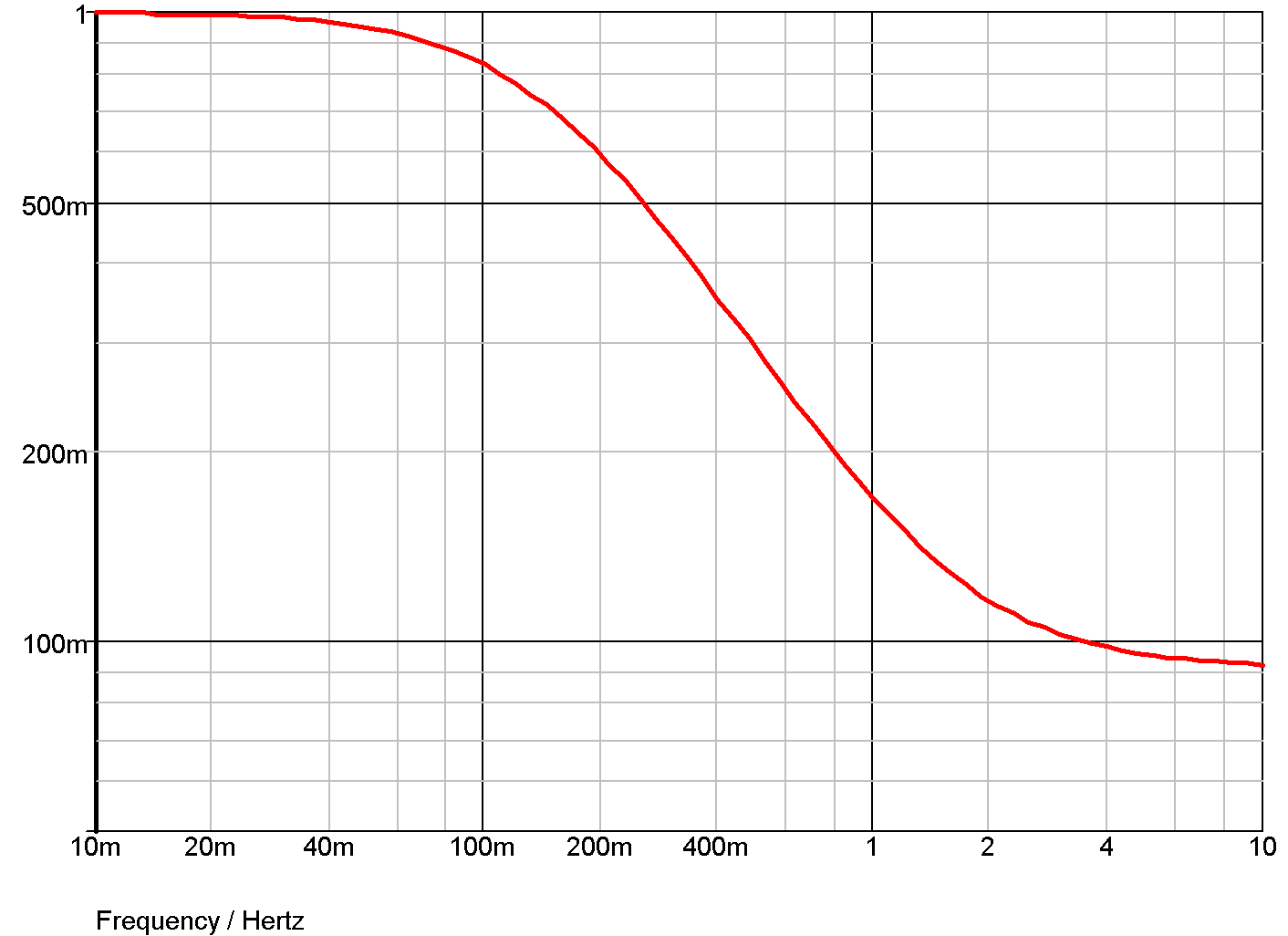
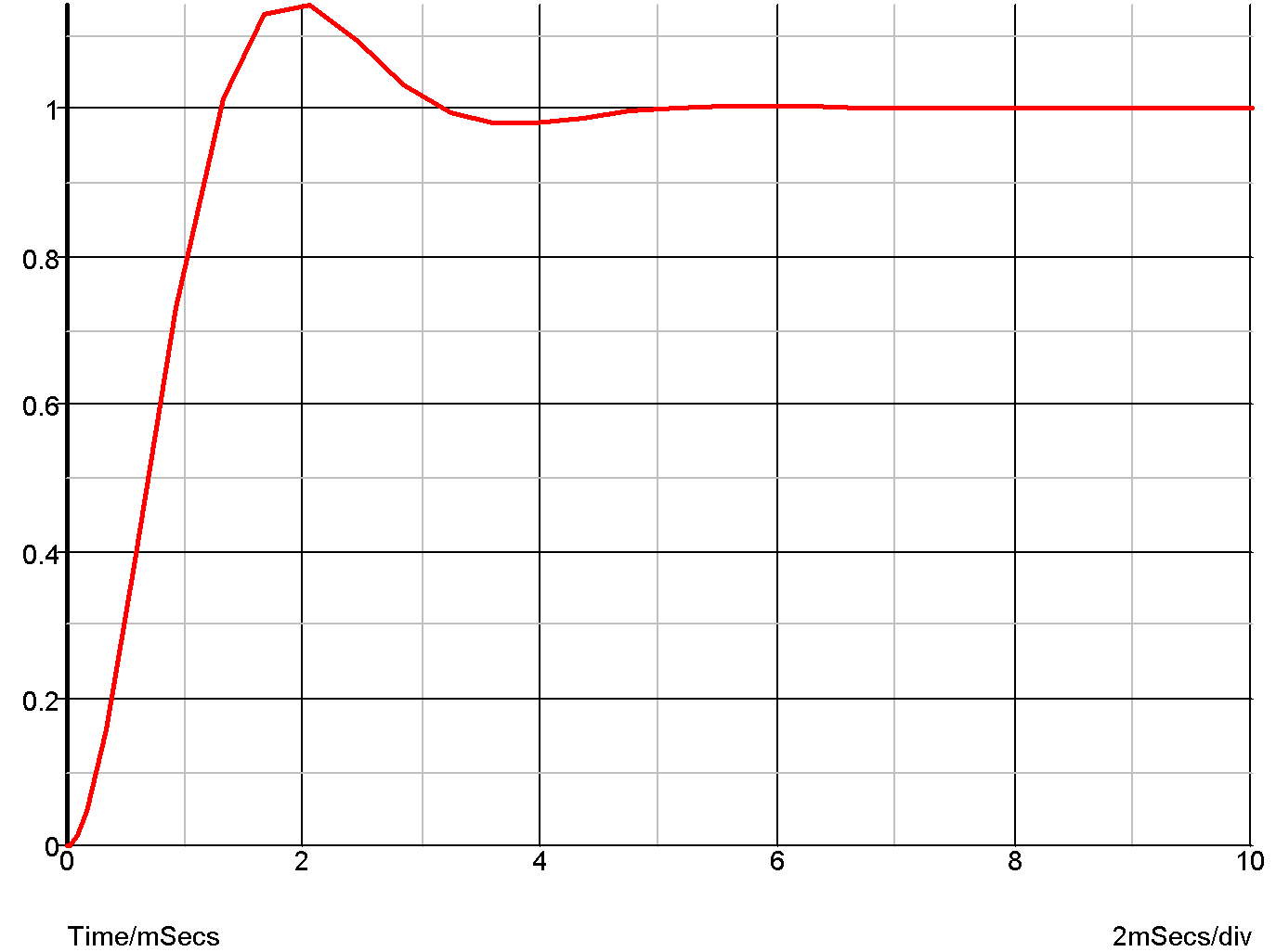
Example 3 - Underdamped second order response
.model Laplace s_xfer
+ laplace="1/(s2+1.1*s+1)"
+ denormalized_freq=2k
The above expression is a second order response that is slightly underdamped. The following graph shows the transient response.
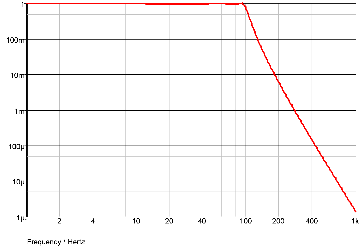
Example 4 - 5th order Chebyshev low-pass filter
The S-domain transfer block has a number of built in functions to implement standard filter response. Here is an example. This is a 5th order chebyshev with -3dB at 100Hz and 0.5dB passband ripple.
.model Laplace s_xfer
+ laplace="chebyshevLP(5,100,0.5)"
+ denormalized_freq=1
and the response:
The Laplace Expression
As seen in the above examples, the transfer function of the device is defined by the model parameter LAPLACE. This is a text string and must be enclosed in double quotation marks. This may be any arithmetic expression containing the following elements:
| Operators: | + - * / \^ where ^ means raise to power. Only integral powers may be specified. | ||||||||||||
| Constants | Any decimal number following normal rules. SPICE style engineering suffixes are accepted. | ||||||||||||
| S Variable | This can be raised to a power with '^' or by simply placing a constant directly after it (with no spaces). E.g. s^2 is the same as s2. | ||||||||||||
| Filter response functions |
These are:
|
||||||||||||
Where:
|
Defining the Laplace Expression Using Coefficients
Instead of entering a Laplace expression as a string, this can also be entered as two arrays of numeric coefficients for the numerator and denominator. In general this is less convenient than entering the expression directly, but has the benefit that it supports the use of parameters. In this method, use the NUM_COEFF and DEN_COEFF parameters instead of the LAPLACE expression.
.param f0=10
.param w0 = {2*3.14159265*f0}

.model laplace s_xfer num_coeff = [1] den_coeff = [{1/w0},1]
Other Model Parameters
- DENORMALISED_FREQ is a frequency scaling factor.
- INT_IC specifies the initial conditions for the device. This is an array of maximum size equal to the order of the denominator. The right-most value is the zero'th order initial condition.
- NUM_COEFF and DEN_COEFF - see Defining the Laplace Expression Using Coefficients.
- GAIN and IN_OFFSET are the DC gain and input offset respectively.
Limitations
SIMetrix expands the expression you enter to create a quotient of two polynomials. If the constant terms of both numerator and denominator are both zero, both are divided by S. That process is repeated until one or both of the polynomials has a non-zero constant term.
The result of this process must satisfy the following:
- The order the denominator must be greater than or equal to that of the numerator.
- The constant term of the denominator may not be zero.
Implementation
This device implements a Laplace transform using a network of integrators. The diagram below shows the configuration used for a third order network.
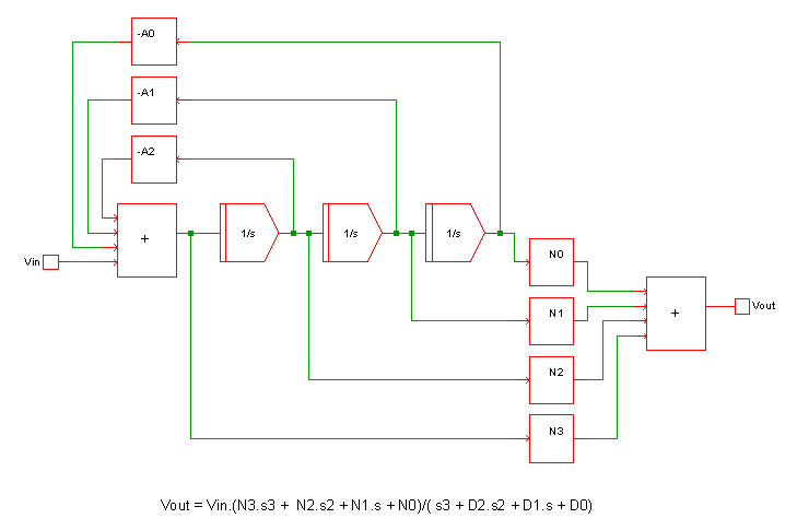 This method can implement a quotient of polynomials in the s variable and any expression that can be reduced to a quotient of polynomials. For such expressions it is fast and efficient.
This method cannot implement expressions containing arbitrary functions such as square-root or exponentials. Such Laplace expressions must be implemented using the convolution method.
| ◄ Junction FET | Laplace Transfer Function - Convolution Implementation ▶ |