Generic Parts
As explained in the overview generic parts are devices that are defined by one or more parameters entered by the user after the part is placed. The following generic parts are available:
| Device | SIMPLIS support? |
| Ideal Transformer | Yes |
| Saturable Inductors and Transformer | No |
| Inductor | Yes |
| Capacitor | Yes |
| Resistor | Yes |
| Potentiometer | Yes |
| Transmission Line (Lossless) | No |
| Transmission Line (Lossy) | No |
| Infinite capacitor | No |
| Infinite inductor | No |
| Voltage source | Yes |
| Current source | Yes |
| Voltage controlled voltage source | Yes |
| Voltage controlled current source | Yes |
| Current controlled voltage source | Yes |
| Current controlled current source | Yes |
| Voltage controlled switch | No |
| Voltage controlled switch with Hysteresis | Yes |
| Delayed Switch | No |
| Parameterised Opamp | Yes |
| Parameterised Opto-coupler | No |
| Parameterised Comparator | No |
| VCO | No |
| Device |
In this topic:
SIMPLIS Primitive Parts
The following parts are only available with the SIMetrix/SIMPLIS product and when in SIMPLIS. They can all be found under the menu . For full details, see the SIMPLIS Reference Manual.
| Device |
| Comparator |
| Set-reset flip-flop |
| Set-reset flip-flop clocked |
| J-K flip-flop |
| D-type flip-flop |
| Toggle flip-flop |
| Latch |
| Simple switch - voltage controlled |
| Simple switch - current controlled |
| Transistor switch - voltage controlled |
| Transistor switch - current controlled |
| VPWL Resistor |
| IPWL Resistor |
| PWL Capacitor |
| PWL Inductor |
Saturable Inductors and Transformers
SIMetrix is supplied with a number of models for inductors and transformers that correctly model saturation and, for most models, hysteresis. As these parts are nearly always custom designed there is no catalogue of manufacturers parts as there is with semiconductor devices. Consequently a little more information is needed to specify one of these devices. This section describes the facilities available and a description of the models available.
Core Materials
The available models cover a range of ferrite and MPP core materials for inductors and transformers with any number of windings. The complete simulation model based on a library core model is generated by the user interface according to the winding specification entered.
Placing and Specifying Parts
-
Select the menu
You will see the following dialog box:
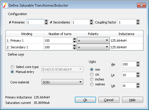
- Specify the number of windings required for primary and secondary in the Configuration section. If you just want a single inductor, set primary turns to 1 and secondaries to 0.
- Specify the number of turns for each winding in the windings list below the Configuration section. You can also define positive or negative polarity which will control the orientation of the winding.
- Specify the coupling factor in the Configuration section. The coupling factor is the same for all windings. You can define different coupling factors for each winding by adding ideal inductors in series with one or more windings. In some instances it may be necessary to add coupled inductors in series. This is explained in more detail in Coupling Factor.
- Specify the core characteristics in the Define Core section. A number of standard core sets are pre-programmed and can be selected from the Select Core Type list at the top. If the part you wish to use is not in the list or if you wish to use a variant with a - say - different air gap, you can manually enter the characteristics by clicking on the Manual Entry check box.
| Ae | Effective Area |
| Le | Effective Length |
| Ue | Relative Permeability |
| Core Material |
Model Details
The models for saturable magnetic parts can be found in the file cores.lb. Most of the models are based on the Jiles-Atherton magnetic model which includes hysteresis effects. The MPP models use a simpler model which does not include hysteresis. These models only define a single inductor. To derive a transformer model, the user interface generates a subcircuit model that constructs a non-magnetic transformer using controlled sources. The inductive element is added to the core which then gives the model its inductive characteristics.
The model does not currently handle other core characteristics such as eddy current losses nor does it handle winding artefacts such as resistive losses, skin effect, inter-winding capacitance or proximity effect.
Ideal Transformers
Ideal transformers may be used in both SIMetrix and SIMPLIS modes. Note that SIMPLIS operation is more efficient if the coupling factors are set to unity.
To define an ideal transformer, select the menu . This will open the following dialog box:
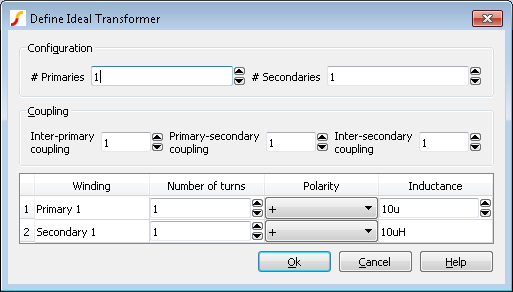
Configuration
Specify the number of primaries and secondaries. You can specify up to 20 of each.
Define winding turns and inductance
Specify the number of turns for each winding in the list at the bottom of the window. Also set the inductance for the first primary. The inductances for the other windings will automatically update. These are calculated from the primary inductance and the relevant turns ratio.
You may also specify the polarity for each winding. The polarity of the winding will be shown on the schematic symbol using the conventional dot at one end of the winding.
Coupling factor
| Inter-primary coupling | Coupling factor between primaries. |
| Inter secondary coupling | Coupling factor between secondaries. |
| Primary-secondary coupling | Coupling factor from each primary to each secondary. |
This method of implementing an ideal transformer is not totally general purpose as you cannot arbitrarily define inter winding coupling factors. If you need a configuration not supported by the above method, you can define any ideal transformer using ideal inductors and the Mutual Inductance device. The SIMetrix version is explained in Mutual Inductors. For the SIMPLIS equivalent, see the SIMPLIS reference manual.
DC Transformers
The DC transformer model is like a normal transformer except that it has - in effect - infinite inductance. So it will work at DC and has zero magnetisation current.
To place a DC transformer, select menu . This will open the following dialog box:
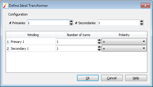
Configuration
Specify the number of primaries and secondaries. You can specify up to 20 of each.
Define winding turns
Define the number of turns for each winding in the list. Note that the behaviour of the part depends only on the ratios between the turns. You may also specify the polarity for each winding. The polarity of the winding will be shown on the schematic symbol using the conventional dot at one end of the winding.
Coupling Factor
The standard user interface for both saturable and ideal transformers provide only limited flexibility to specify inter-winding coupling factor. In the majority of applications, coupling factor is not an important issue and so the standard model will suffice.
In some applications, however, the relative coupling factors of different windings can be important. An example is in a flyback switched mode supply where the output voltage is sensed by an auxiliary winding. In this instance, best performance is achieved if the sense winding is strongly coupled to the secondary. Such a transformer is likely to have a different coupling factor for the various windings.
You can use external leakage inductances to model coupling factor and this will provide some additional flexibility. One approach is to set the user interface coupling factor to unity and model all non-ideal coupling using external inductors. In some cases it may be necessary to couple the leakage inductors. Consider for example an E-core with 4 windings, one on each outer leg and two on the inner leg. Each winding taken on its own would have approximately the same coupling to the core and so each would have the same leakage inductance. But the two windings on the centre leg would be more closely coupled to each other than to the other windings. To model this, the leakage inductances for the centre windings could be coupled to each other using the mutual inductor method described in the next section.
Mutual Inductors
You can specify coupling between any number of ideal inductors, using the mutual inductor device. There is no menu or schematic symbol for this. It is defined by a line of text that must be added to the netlist. (See Manual Entry of Simulator Commands). The format for the mutual inductance line is:
Kxxxx inductor_1 inductor_2 coupling_factor
| inductor_1 | Part reference of the first inductor to be coupled. |
| inductor_2 | Part reference of the second inductor to be coupled. |
| coupling_factor | Value between 0 and 1 which defines strength of coupling. |
Note
If more than 2 inductors are to be coupled, there must be a K device to define every possible pair.
Examples
** Couple L1 and L2 together
K12 L1 L2 0.98
** Couple L1, L2 and L3
K12 L1 L2 0.98
K23 L2 L3 0.98
K13 L1 L3 0.98
Resistors
Resistors may be used in both SIMetrix and SIMPLIS modes. Note that in SIMetrix mode a number of additional parameters may be specified. These will not work with SIMPLIS and must not be specified if dual mode operation is required.
Select from menu.
To edit value use F7 or select popup menu Edit Part...
menu as usual. This will display the following dialog for resistors.
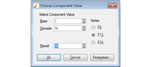 You can enter the value directly in the Result
box or use the Base
and Decade
up/down controls.
You can enter the value directly in the Result
box or use the Base
and Decade
up/down controls.
Additional Parameters
Press Parameters... button to edit additional parameter associated with the device such as temperature coefficients (TC1, TC2). Refer to device in the Simulator Reference Manual for details of all device parameters.
Ideal Capacitors and Inductors
Capacitors and inductors may be used in both SIMetrix and SIMPLIS modes. Note that in SIMetrix mode a number of additional parameters may be specified. These will not work with SIMPLIS and must not be specified if dual mode operation is required.
The following dialog will be displayed when you edit a capacitor or inductor:
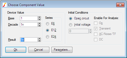
The device value is edited in the same manner as for resistors. You can also supply an initial condition that defines how the device behaves while a DC operating point is calculated. For capacitors you can either specify that the device is open circuit or alternatively you can specify a fixed voltage. For inductors, the device can be treated as a short circuit or you can define a constant current.
Infinite Capacitors and Inductors
The infinite capacitors and inductors are often useful for AC analysis.
To place an infinite capacitor, select menu To place an infinite inductor, select menu
The infinite capacitor works as follows:
- During the DC bias point calculation, it behaves like an open circuit, just like a regular finite capacitor.
- During any subsequent analysis it behaves like a voltage source with a value equal to the voltage achieved during the DC bias point calculation.
- During the DC bias point calculation, it behaves like a short circuit, just like a regular finite inductor.
- During any subsequent analysis it behaves like a current source with a value equal to the current achieved during the DC bias point calculation.
The infinite capacitor is a built in primitive part and is actually implemented by the voltage source device. The infinite inductor is a subcircuit using an infinite capacitor and some controlled sources.
Multi-Level Capacitors
The Multi-Level Capacitor has four model levels. As the level increases, additional parasitic circuit elements are added. This capacitor, available with Version 8.0 or later, is used to model a wide variety of capacitor types where the number and type of parasitic circuit elements can be configured.
| Model Name: | Multi-Level Capacitor (Level 0-3 w/Quantity) |
| Simulator: | This device is compatible with both the SIMetrix and SIMPLIS simulators |
| Parts Selector Menu Location (SIMetrix): | |
| Parts Selector Menu Location (SIMetrix): | |
| Parts Selector Menu Location (SIMetrix): | |
| Parts Selector Menu Location (SIMPLIS): | |
| Symbol Library: | passives.sxslb |
| Model File (SIMetrix): | preproc.lb |
| Model File (SIMPLIS): | simplis_param.lb |
| Subcircuit Name: | MULTI_LEVEL_CAP_QTY |
| Multiple Selections: | Multiple devices can be selected and edited simultaneously |
Editing the Multi-Level Capacitor
- Double click the symbol on the schematic to open the editing dialog to the Parameters tab.
- Choose a model level, and then make the appropriate changes to the fields described in the table below the image.
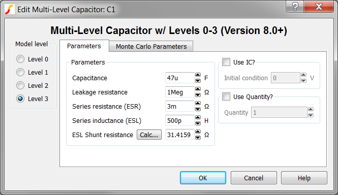
| Label | Levels | Units | Description |
| Capacitance | 0,1,2,3 | F | Capacitance value |
| Leakage resistance | 1,2,3 | ???MATH???\Omega???MATH??? | Leakage resistance across the capacitor |
| Series resistance (ESR) | 2,3 | ???MATH???\Omega???MATH??? | The equivalent series resistance (ESR) |
| Series inductance (ESL) | 3 | H | The equivalent series inductance (ESL) |
| ESL Shunt resistance | 3 | ???MATH???\Omega???MATH??? | The shunt resistance in parallel with the ESL. This resistance is included to limit the maximum frequency response of the parasitic ESL, which maximizes the simulation speed in SIMPLIS mode. Click Calc... to calculate this value. |
| Use IC? | all | n/a |
|
| Initial condition | all | V | Initial voltage of the capacitor at time=0 |
| Use Quantity? | all | n/a | If checked, the model uses the specified Quantity of capacitors in parallel. |
| Quantity | all | n/a | Number of capacitors in parallel. Note: To maximize simulation speed when using SIMPLIS, place a single symbol and specify a value for this parameter instead of placing multiple capacitors. |
- Click on the Monte Carlo Parameters tab.
- Make the appropriate changes to the fields described in the table below the image.
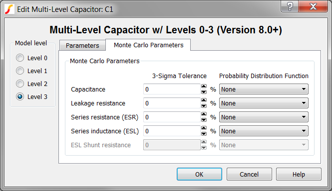
| Label | Levels | Units | Description |
| Capacitance | 0,1,2,3 | % | 3-sigma tolerance for the capacitance value |
| Leakage resistance | 1,2,3 | % | 3-sigma tolerance for the leakage resistance across the capacitor |
| Series resistance (ESR) | 2,3 | % | 3-sigma tolerance for the equivalent series resistance (ESR) |
| Series inductance (ESL) | 3 | % | 3-sigma tolerance for the equivalent series inductance (ESL) |
| Probability Distribution Function | all | n/a |
The choices for this function for each available parameter are the following:
|
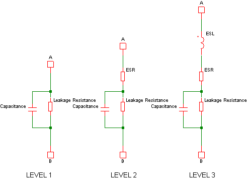
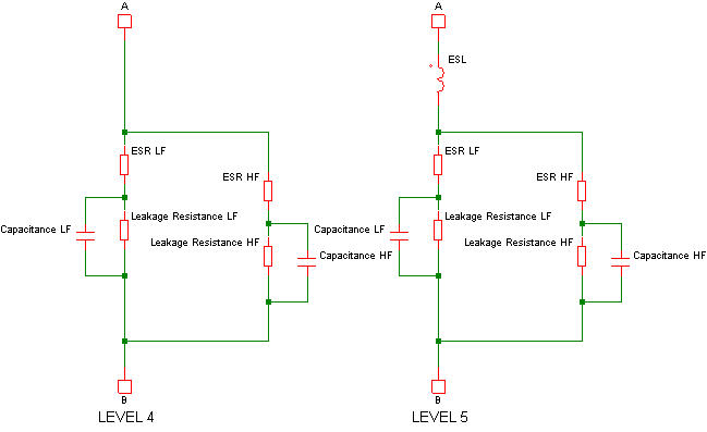
Multi-Level Capacitor Model Levels
The Multi-Level capacitor has four levels: 0, 1, 2, and 3. As the model level increases, additional parasitic circuit elements are added to the model.
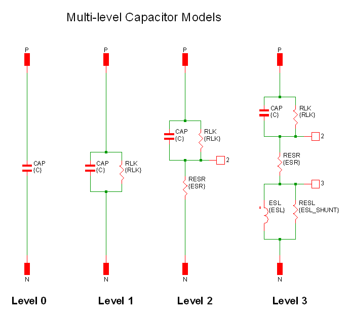 The following table summarises the model parameters:
| Parameter | Levels | Description |
| CAP | all | Linear capacitance |
| RLK | 1,2,3 | Leakage resistance |
| RESR | 2,3 | Equivalent series resistance |
| LESL | 3 | Equivalent series inductance |
| RESL | 3 | ESL shunt resistance |
Quantity Implementation - SIMPLIS Mode
The Multi-Level Capacitor model has two quantity parameters, USE_QTY and QTY, which specify the number of capacitors in parallel.
Configuring these parameters minimizes the number of reactive circuit elements in the model and, therefore, provides a maximum simulation speed.
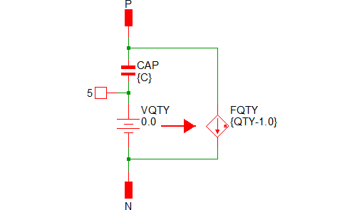
The implementation of the quantity parameter uses a "DC Transformer" technique where the capacitor's terminal current is multiplied by a constant using a Current Controlled Current Source (CCCS). This technique effectively divides all resistance and inductance values by the quantity parameter (QTY) and multiplies the capacitance by that same value. This circuitry is added if the USE_QTY parameter is set to 1.
A schematic of the quantity implementation for a Level 0 Multi-Level Capacitor is shown below:
Quantity Implementation - SIMetrix Mode
In SIMetrix, the quantity parameter is implemented with the "M" parameter which is common to the primitive SPICE components. This improves SIMetrix simulation speed and correctly scales resistances for noise analysis.
Electrolytic Capacitors
The electrolytic capacitor model has been superseded by the Multi-level Capacitor. The electrolytic capacitor is still available from the parts selector at locations Passives -> Capacitors, Simple (Legacy) and Passives -> Capacitors, Detailed (Legacy)
 |
Simple Model |
 |
Detailed Model |
Passives -> Capacitors, Simple (Legacy)
Potentiometer
The potentiometer may be used in both SIMetrix and SIMPLIS modes. To place, select the menu . This device can be edited in the usual manner with F7/Edit Part...
popup. This will display:
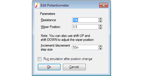 Enter Resistance and Wiper position as required.
Check Run simulation after position change if you wish a new simulation to be run immediately after the wiper position changes.
The potentiometer's wiper position may also be altered using the shift-up and shift-down keys while the device is selected. Edit Inc/dec step size to alter the step size used for this feature.
Lossless Transmission Line
Select from menu or press hot key 'T'. Editing in the usual way will display:
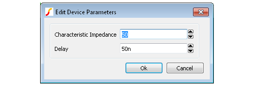 Enter the Characteristic Impedance (Z0) and Delay as indicated.
Lossy Transmission Line
Select from menu . Editing in the usual way will display:
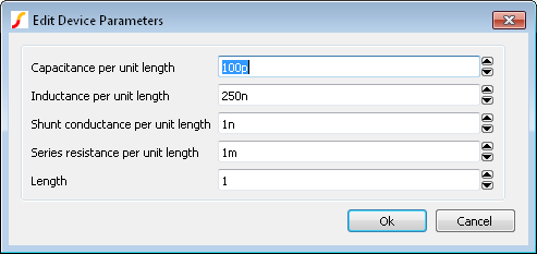 Lossy lines must be defined in terms of their per unit length impedance characteristics.
The lossy line model is implemented in a subcircuit that uses the Laplace transfer device. See Laplace Transfer Function for details.
Fixed Voltage and Current Sources
See Circuit Stimulus.
Controlled Sources
There are four types which can be found under menu :
- Voltage controlled voltage source or VCVS
- Voltage controlled current source or VCCS
- Current controlled voltage source or CCVS
- Current controlled current source or CCCS
These have a variety of uses. A VCVS can implement an ideal opamp; current controlled devices can monitor current; voltage controlled devices can convert a differential signal to single ended.
They require just one value to define them which is their gain. Edit value in the usual way and you will be presented with a dialog similar to that used for resistors, capacitors and inductors but without the Parameters... button.
Voltage Controlled Switch
This is essentially a voltage controlled resistor with two terminals for the resistance and two control terminals. Place one on the schematic with . Editing using F7 or equivalent menu displays:
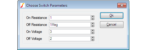
If On Voltage > Off Voltage
If control voltage > On Voltage
Resistance = On Resistance
else if control voltage < Off Voltage
Resistance = Off Resistance
If Off Voltage > On Voltage
If control voltage > Off Voltage
Resistance = Off Resistance
else if control voltage < On Voltage
Resistance = On Resistance
If the control voltage lies between the On Voltage and Off Voltage the resistance will be somewhere between the on and off resistances using a law that assures a smooth transition between the on and off states. Refer to Simulator Reference Manual/Analog Device Reference/Voltage Controlled Switch
Switch with Hysteresis
An alternative switch device is available which abruptly switches between states rather than following a continuous V-I characteristic. This device can be used with both SIMetrix and SIMPLIS although the behaviour is slightly different in each. The switching thresholds are governed by an hysteresis law and, when used with the SIMetrix simulator, the state change is controlled to occur over a defined time period which can be edited.
This device can be placed on a schematic with the menu .
Parameters are:
| Parameter | Description |
| Off Resistance | Switch resistance in OFF state. |
| On Resistance | Switch resistance in ON state. |
| Threshold | Average threshold. Switches to on state at this value plus half the hysteresis. Switch to off state at this value less half the hysteresis. |
| Hysteresis | Difference between upper and lower thresholds. |
| Switching Time | Time switch takes to switch on. Note that this is the total time from the point at which the switch starts to switch on to the point when it is fully switched on. |
| Initial condition | Sets the initial state of the switch at the start of the simulation. |
If you need to control switch on times and switch off times independently, you can use the delayed switch model. See Delayed Switch.
Delayed Switch
Implements a voltage-controlled switch with defined on and off delay. This model can be used to implement relays. Switch action is similar to the Switch with Hysteresis described above. The delayed switch model has all the functionality of the hysteresis switch with the addition of time delay parameters and separate parameters for switch on and switch off times. Unlike the hysteresis switch, this device does not have an exact SIMPLIS equivalent.
This device can be placed on a schematic with the menu .
Parameters are:
| Parameter | Description |
| Off Resistance | Switch resistance in OFF state |
| On Resistance | Switch resistance in ON state |
| Threshold Low | Switch switches off when control voltage drops below this threshold |
| Threshold High | Switch switches on when control voltage rises above this threshold |
| On Delay | Delay between high threshold being reached and switch starting to switch on |
| Off Delay | Delay between low threshold being reached and switch starting to switch off |
| Switching Time (On) | Total time switch takes to switch on |
| Switching Time (Off) | Total time switch takes to switch off |
Parameterised Opamp
Implements an operational amplifier and is available from menu This is available from menu It is defined by the parameters listed below.
| Parameter | units | Description |
| Offset Voltage | V | Input voltage needed for zero output |
| Bias Current | A | Average of input currents when out=0 |
| Offset Current | A | Difference between input currents when out=0 |
| Open-loop gain | Vout/(Vin+ - Vin-) (Simple ratio - not dB) | |
| Gain-bandwidth | Hz | Gain x bandwidth product |
| Pos. Slew Rate | V/s | Slew rate for positive output transistions |
| Neg. Slew Rate | V/s | Slew rate for negative output transistions(SIMPLIS only. In SIMetrix the negative slew rate is the same as the positive slew rate) |
| CMRR | Common mode rejection ratio. Expressed as straight ratio - not in dB | |
| PSRR | Power supply rejection ratio. Expressed as straight ratio - not in dB | |
| Input Resistance | ???MATH???\Omega???MATH??? | Differential input resistance |
| Output Res. | ???MATH???\Omega???MATH??? |
Series output resistance. For SIMetrix this interacts with the quiescent current; The output resistance must satisfy:
Rout > 0.0129/IQWhere IQ is the Quiescent current. If the above is not satisfied, there is a high risk that the model will not converge. This limitation is a consequence of the way the output stage is implemented. The limitation does not apply to SIMPLIS |
| Quiescent Curr. | A | Supply current with no load. This must satisfy the relation shown in Output Res. above |
| Headroom Pos. | V | Difference between positive supply voltage and maximum output voltage |
| Headroom Neg. | V | Difference between minimum output voltage and negative supply rail. |
| Offset V. (Statistical) | V | For Monte-Carlo analysis only. Specifies the 1-sigma offset voltage tolerance. (SIMetrix only) |
Parameterised Opto-coupler
Implements a 2-in 2-out optically isolated coupler. This is available from menu It is defined by just two parameters described in the following table:
| Parameter | Description |
| Current transfer ratio | Ratio between output current and input current |
| Roll-off frequency | -3dB point |
Parameterised Comparator
Implements a simple differential comparator. This is available from menu Its parameters are defined in the following table:
| Parameter | Description |
| Input Resistance | Differential input resistance. |
| Output Resistance | Series output resistance. |
| Hysteresis | Difference between switching tresholds. The output will switch from low-high when the differential input voltage rises above half the hysteresis. The output will switch from high-low when the differential input voltage falls below half the hysteresis. |
| Output Low Voltage | Unloaded output voltage in low state. |
| Output High Voltage | Unloaded output voltage in high state. |
| Delay | Delay between threshold crossing and start of the output changing state. |
| Rise/Fall Time | Output rise and fall time. |
VCO
Implements a simple voltage controlled oscillator with a digital output. You can place a VCO on the schematic using menu Its parameters are:
| Parameter | Description |
| Frequency at VC=0 | Output frequency for a control voltage of zero |
| Gain Hz/V | Change in frequency vs change in input voltage |
Verilog-A Library
If you have a SIMetrix Pro or SIMetrix Elite you may also use one of the Verilog-A implemented devices available under the These devices are defined using the Verilog-A language. The Verilog-A code for these devices may be found in the support\ valibrary directory under the SIMetrix root.
Currently there are 4 Verilog-A library devices as described in the following paragraphs.
Voltage Controlled Delay
Implements a variable analog delay.
This device has three parameters as defined in the table below. Double click the device to edit its parameters.
| Parameter | Description |
| Max delay | The maximum delay that the device may provide in seconds. |
| Voltage for minimum delay | Input voltage for minimum delay (i.e. zero) |
| Voltage for maximum delay | Input voltage for maximum delay. The delay when between the minimum and maximum voltages will be calculated following a linear characteristic. |
Fixed Delay
Implements a fixed analog delay
This device has just a single parameter defining its delay in seconds. Double click the device to edit.
Sinewave VCO
Implements a sinewave voltage controlled oscillator. This has four parameters as defined below:
| Parameter | Description |
| Amplitude | Peak amplitude of sine wave. |
| Centre Frequency | Frequency for zero volts input. |
| Gain Hz/Volt | Change in frequency for each volt change in the input. |
| Minimum steps per cycle | Minimum number of time points per cycle. The simulator will force time points to ensure that each cycle has at least the number specified. |
Pulse Width Modulator
Implements a voltage controlled pulse width. Defined by 6 parameters as follows:
| Parameter | Description |
| Frequency | Frequency of pulse |
| Input low voltage | Voltage for zero duty cycle |
| Input high voltage | Voltage for maximum duty cycle |
| Output low voltage | Low voltage of output pulse |
| Output high voltage | High voltage of output pulse |
| Maximum duty cycle | Maximum duty cycle. This may not be higher than 0.999 |
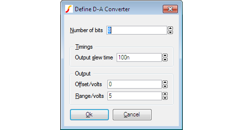
Generic ADCs and DACs
Generic data conversion devices are available from the menus and
 These devices are implemented using the simulator's ADC and DAC models. For details of these refer to Simulator Reference Manual/Digital Mixed Signal Device Reference/Analog-Digital Converter and Simulator Reference Manual/Digital Mixed Signal Device Reference/Digital-Analog Converter
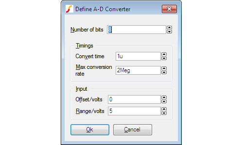
The controls in these boxes are explained below.
Number of bits
Resolution of converter. Values from 1 to32
Convert time (ADC)
Time from start convert active (rising edge) to data becoming available
Max conversion rate (ADC)
Max frequency of start convert. Period (1/f) must be less than or equal to convert time.
Output slew time
Whenever the input code changes, the output is set on a trajectory to reach the target value in the time specified by this value.
Offset voltage
Self-explanatory.
Range
Full scale range in volts.
Generic Digital Devices
A number of generic digital devices are provided on the menu. Each will automatically create a symbol using a basic spec. provided by your entries to a dialog box. Functions provided are, counter, shift register, AND, OR, NAND and NOR gates, and bus register.
Arbitrary Non-linear Passive Devices
Each of these will place a part which looks exactly like its linear counterpart. The difference is that when you try and edit its value with F7 or menu Edit Part... you will be prompted to enter an expression. In the case of the resistor and capacitor, this relates its value to the applied voltage and for inductor the expression relates its inductance to its current. For resistors and capacitors, the terminal voltage is referred in the equation as 'V(N1)' and for inductors the device's current is referred to as 'I(V1)'.
| ◄ Circuit Stimulus | Creating Models ▶ |