Current Controlled Current Source
In this topic:
Netlist Entry
Linear Source
Fxxxx nout+ nout- vc current_gain [GOUT=output_conductance]
| nout+ | Positive output node |
| nout- | Negative output node |
| vc | Controlling voltage source |
| current_gain | Output current/Input current |
| output_conductance | Conductance at output terminals |
GOUT has a default value of zero unless the PSPICEGMIN option is set in which case it has a default value of GMIN. GMIN is set using ".OPTIONS GMIN=value" and has a default value of 1e-12.
SPICE2 polynomial sources are also supported in order to maintain compatibility with commercially available libraries for IC's. (Most operational amplifier models for example use several polynomial sources). In general, however the arbitrary source (see Arbitrary Source) is more flexible and easier to use.
Polynomial Source
Fxxxx nout+ nout- POLY( num_inputs ) vc1 vc2 ...
+ polynomial_specification
| vc1, vc2 | Controlling voltage sources |
| num_inputs | Number of controlling currents for source. |
| polynomial_specification | See Polynomial Specification. |
The specification of the controlling voltage source or source requires additional netlist lines. The schematic netlister automatically generates these for the four terminal device supplied in the symbol library.
Example
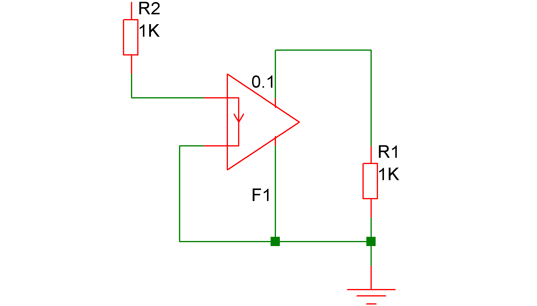
In the above circuit, the current in the output of F1 (flowing from top to bottom) will be 0.1 times the current in R2.
Polynomial Specification
The following is an extract from the SPICE2G.6 user manual explaining polynomial sources.
SPICE allows circuits to contain dependent sources characterised by any of the four equations
- i=f(v)
- v=f(v)
- i=f(i)
- v=f(i)
where the functions must be polynomials, and the arguments may be multidimensional. The polynomial functions are specified by a set of coefficients p0, p1, ..., pn. Both the number of dimensions and the number of coefficients are arbitrary. The meaning of the coefficients depends upon the dimension of the polynomial, as shown in the following examples:
Suppose that the function is one-dimensional (that is, a function of one argument). Then the function value fv is determined by the following expression in fa (the function argument):
\[ fv = p0 + (p1.fa) + (p2.fa^2) + (p3.fa^3) + (p4.fa^4) + (p5.fa^5) + ... \]
Suppose now that the function is two-dimensional, with arguments fa and fb. Then the function value fv is determined by the following expression:
\[ \begin{split} fv = p0 + (p1.fa) + (p2.fb) + (p3.fa^2) + (p4.fa.fb) + (p5.fb^2) \\ + (p6.fa^3) + (p7.fa^2.fb) + (p8.fa.fb^2) + (p9.fb^3) + ... \end{split} \]
Consider now the case of a three-dimensional polynomial function with arguments fa, fb, and fc. Then the function value fv is determined by the following expression:
\[ \begin{split} fv = p0 + (p1.fa) + (p2.fb) + (p3.fc) + (p4.fa^2) + (p5.fa.fb) + (p6.fa.fc) + (p7.fb^2) + (p8.fb.fc) \\ + (p9.fc^2) + (p10.fa^3) + (p11.fa^2.fb) + (p12.fa^2.fc) + (p13.fa.fb^2) + (p14.fa.fb.fc) \\ + (p15.fa.fc^2) + (p16.fb^3) + (p17.fb^2.fc) + (p18.fb.fc^2) + (p19.fc^3) + (p20.fa^4) + ... \end{split} \]
| Note | If the polynomial is one-dimensional and exactly one coefficient is specified, then SPICE assumes it to be p1 (and p0 = 0.0), in order to facilitate the input of linear controlled sources. |
| ◄ Capacitor | Current Controlled Voltage Source ▶ |