Curve Measurements
In this topic:
Overview
A number of measurements can be applied to selected curves. The results of these measurements are displayed in the measurement window below the main graph drawing area. See Elements of the Graph Window.
Some of these measurements can be selected from the tool bar while the remainder may be accessed via the menu or by pressing F3.
Measurement functions may also be applied to Fixed Probes so that they are automatically updated when a simulation is repeated. See Applying Measurements to Fixed Probes for more details.
In general to perform a measurement, select the curve or curves then select measurement from tool bar or menu. If there is only one curve displayed, it is not necessary to select it.
Available Measurements
A wide range of measurement functions are available. Select menu to see the complete list. For more information see Using the Define Measurement GUI.
Using the Define Measurement GUI
The Define Measurement GUI is a general purpose interface to the measurement system and provides access to all measurement functions along with a means to define custom measurements.
To open the Define Measurement GUI, select menu You will see the following dialog box:
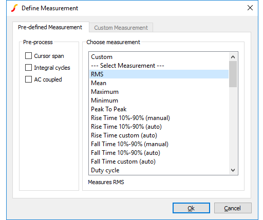
Choose measurement
Lists all available measurement functions. If cursors are not switched on, some of the functions will be greyed out. These are functions that require you to identify parts of the waveform to be measured. For example the manual rise and fall time measurements require you to mark points before and after the rising or falling edge of interest.
When you click on one of the measurements, some notes will appear at the bottom explaining the measurement and how to use it.
Pre-process
Listed in the pre-process box are three operations that can optionally be performed on the waveform before the measurement function is applied. These are
| Cursor span | Truncates the waveform data to the span defined by the current positions of the cursors. In other words, the measurement is performed on the range defined by the cursor positions. |
| Integral cycles | Truncates the waveform data to an integral number of whole cycles. This is useful for measurements such as RMS which are only meaningful if applied to a whole number of cycles. |
| AC coupled | Offsets the data by the mean value. This is equivalent to 'ACcoupling' the data. |
The above operations are performed in the order listed. So for example, the data is truncated to the cursor span before AC coupling.
Custom Measurement
If you select the Custom entry in the Choose measurement list, the Custom measurement tab will be enabled.
The Custom measurement tab allows you to define your own measurement along with an option to add it to the list of pre-defined measurements. The following explains the entries in the Custom measurement tab.
| Label as displayed on graph | This is the label that will appear alongside the measurement value in the graph legend panel. Usually, this would be literal text, but you may also enter a template string using special variables and script functions. See Templates for details. |
| Expression | Expression to define measurement. Use the variable 'data' to access the data for the curve being measured. The expression must return a single value (i.e. a scalar). See Goal Functions for details of functions that may be used to define measurement expressions. |
| Format template | Defines how the value will be displayed. If you leave this blank, a default will be used which will display the result of the expression along with its units if any. See Templates for details. |
| Save definition to pre-defined measurements | If checked, the measurement definition will be saved to the list shown in pre-defined measurements. You can optionally enter some further details under Save definition. Note that the definition will not appear in the pre-defined list until the dialog is closed an reopened. Further management of custom measurement definitions can be made using the Measurement Definitions Manager. |
| Short description | This is what will be displayed in the list box under Choose measurement in the Pre-defined Measurement tab. |
| Full description | This is what will be displayed below the list box when the item is selected. |
Measurement Definitions Manager
Select menu This will open the Measurement Definitions Manager dialog box shown below:
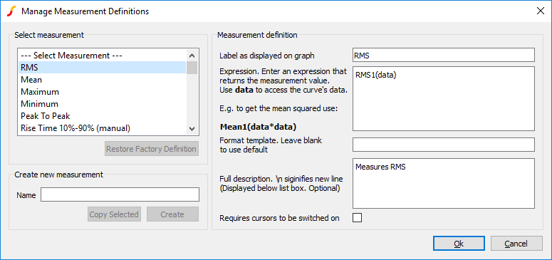
The Measurement Definitions Manager allows you to edit both built in and custom measurement definitions.
Select measurement
Select measurement you wish to edit from this list.
Restore Factory Definition
This button will be enabled for any built-in definition that has been edited in some way. Press it to restore the definition to its original. For custom definitions, this button's label changes to Delete. Press it to delete the definition.
It is not possible to delete built-in definitions
Create new measurement
You can create a completely new empty measurement or you can copy an existing one to edit. Enter a name then press Create to create a new empty definition. To copy an existing definition, select the definition under Select measurement then press Copy selected.
Measurement definition
Define measurement. There are five entries:
| Label as displayed on graph | This is the label that will appear alongside the measurement value in the graph legend panel. Usually, this would be literal text, but you may also enter a template string using special variables and script functions. See Templates for details. |
| Expression | Expression to define measurement. Use the variable 'data' to access the data for the curve being measured. The expression must return a single value (i.e. a scalar). See Goal Functions for details of functions that may be used to define measurement expressions. |
| Format template | Defines how the value will be displayed. If you leave this blank, a default will be used which will display the result of the expression along with its units if any. See Templates for details. |
| Save definition to pre-defined measurements | If checked, the measurement definition will be saved to the list shown in pre-defined measurements. You can optionally enter some further details under Save definition. Note that the definition will not appear in the pre-defined list until the dialog is closed an reopened. Further management of custom measurement definitions can be made using the Measurement Definitions Manager. |
| Full description | This is what will be displayed below the list box when the item is selected. |
| Requires cursors to be switched on | If checked, the measurement will be disabled unless graph cursors are enabled |
Templates
Both the graph label and Format template may be entered using a template containing special variables and expressions. The following is available:
| %yn% | Where n is a number from 1 to 5. y-value returned by expression. The value returned by the expression may be a vector with up to 5 elements. %y1% returns element 1, %y2% returns element 2 etc. |
| %xn% | Where n is a number from 1 to 5. x-value returned by expression. The value returned by the expression may be a vector with up to 5 elements. %x1% returns the x-value of element 1, %x2% returns the x-value of element 2 etc. The xvalues are the values used for the x-axis. You should be aware that not all functions return x-data. |
| %uyn% | The units of the y values. |
| %uxn% | The units of the x values. |
| %% | Literal % character. |
| { expression } | expression will be evaluated and substituted. expression may contain any valid and meaningful script function. For full details, see Script Reference Manual/Function Reference. |
Repeating the Same Measurement
The menu Measure | Repeat Last Measurement will repeat the most recent measurement performed.
Applying Measurements to Fixed Probes
- Select the probe then right click menu Edit/Add Measurements...
-
The following box should be displayed:
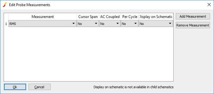
- To begin with a single measurement is shown. Using the drop down box in the Measurement column, select the desired measurement type
-
You may also change some of the attributes:
- Cursor Span specifies that the measurement will be calculated over the current cursor range. If cursors are not switched on, this will be ignored.
- AC coupled specifies that the data will have its DC component removed before the measurement is made.
- Per Cycle will apply an algorithm to detect whole numbers of cycles and apply the measurement over that range.
- Display on schematic will additionally display the measurement result on the schematic using a label attached to the probe.
- To add additional measurements, click the Add Measurement button. A new line will appear. There is no limit to the number of measurements that may be applied.
- To remove a measurement, select the line to be removed then click Remove Measurement.
Notes on Curve Measurement Algorithms
Some of the measurements algorithms make some assumptions about the wave shape being analysed. These work well in most cases but are not fool-proof. The following notes describe how the algorithms work and what their limitations are.
All the measurement algorithms are implemented by internal scripts. The full source of these scripts can be found on the install CD (see Install CD).
'per Cycle' and Frequency Measurements
These measurements assume that the curve being analysed is repetitive and of a fixed frequency. The results may not be very meaningful if the waveform is of varying frequency or is of a burst nature. The /cycle measurements calculate over as many whole cycles as possible.
Each of these measurements use an algorithm to determine the location of x-axis crossings of the waveform. The algorithm is quite sophisticated and works very reliably. The bulk of this algorithm is concerned with finding an optimum base line to use for x-axis crossings.
The per cycle measurements are useful when the simulated span does not cover a whole number of cycles. Measurements such as RMS on a repetitive waveform only have a useful meaning if calculated over a whole number of cycles. If the simulated span does cover a whole number of cycles, then the full version of the measurement will yield an accurate result.
Rise and Fall Time, and Overshoot Measurements
These measurements have to determine the waveforms pulse peaks. A histogram method is used to do this. Flat areas of a waveform produce peaks on a histogram. The method is very reliable and is tolerant of a large number of typical pulse artefacts such as ringing and overshoot. For some wave-shapes, the pulse peaks are not well enough defined to give a reliable answer. In these cases the measurement will fail and an error will be reported.
Distortion
This calculates residue after the fundamental has been removed using an FFT based method. This algorithm needs a reasonable number of cycles to obtain an accurate result. The frequency of the fundamental is displayed in the message window. Note that most frequency components between 0Hz and just before the second harmonic are excluded. The precision of the method can be tested by performing the measurement on a test circuit such as:
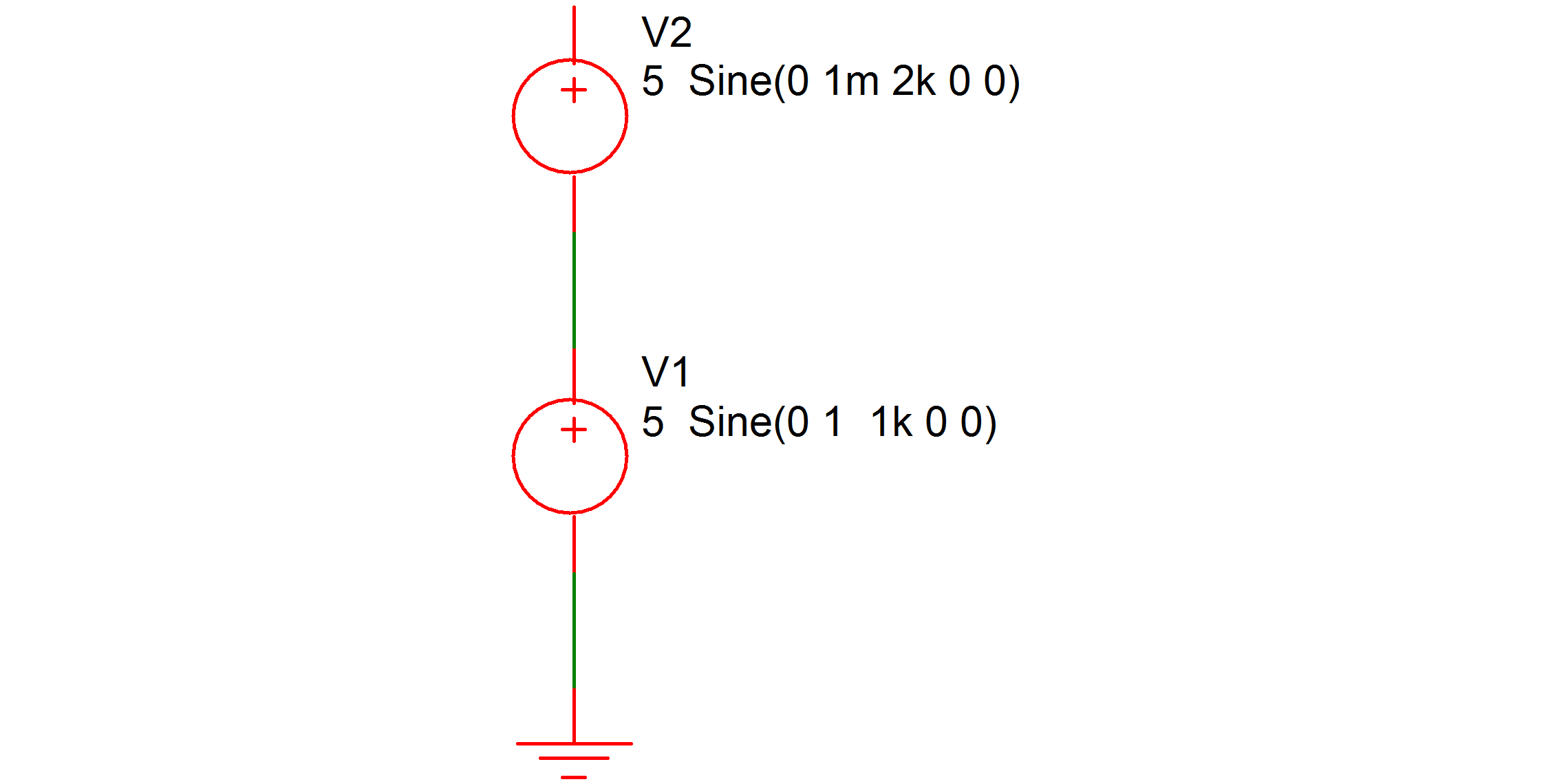
The signal on the pos side of V2 has 0.1% distortion. Use V1 as your main test source (assuming you are testing an amplifier) then after the simulation is complete, check that the distortion measurement of V2 is 0.1%. If it is inaccurate, you will need either to increase the number of measurement cycles or reduce the maximum time step or both. You can adjust the amplitude of V2 appropriately if the required resolution is greater or less than 0.1%.
Note, that in general, accuracies of better than around 1% will require tightening of the simulation tolerance parameters. In most cases just reducing RELTOL (relative tolerance) is sufficient. This can be done from the Options tab of the Choose Analysis Dialog ( ). For a more detailed discussion on accuracy see the chapter "Convergence and Accuracy" in the Simulator Reference Manual.
Frequency Response Calculations
These must find the passband for their calculations. Like rise and fall a histogram approach is used to find its approximate range and magnitude. Further processing is performed to find its exact magnitude.
Note that the algorithms allow a certain amount of ripple in the passband which will work in most cases but will fail if this in excess of about 3dB.
Note that the frequency response measurements are general purpose and are required to account for a wide variety of responses including those with both high and low pass elements as well as responses with band pass ripple. This requirement compromises accuracy in simpler cases. So, for example, to calculate the -3dB point of a low pass response that extends to DC, the 0dB point is taken to be a point midway between the start frequency and the frequency at which roll-off starts. A better location would be the start frequency but this would be inaccurate if there was a high pass roll off at low frequencies. Taking the middle point is a compromise which produces good - but not necessarily perfect - results in a wide range of cases. To increase accuracy in the case described above, start the analysis at a lower frequency, this will lower the frequency at which the 0dB reference is taken.
Plots from curves
Two plots can be made directly from selected curves. These are described below
FFT of Selected Curve
With a single curve selected, select menu . A new graph sheet will be opened with the FFT of the curve displayed. To plot an FFT of the curve over the span defined by the cursor locations select menu .
Smoothed Curves
With a single curve selected, select one of the menus. For you will need to enter a time constant value. A new curve will be displayed which is a filtered version of the selected curve.
The above functions will still work if you don't select any curves. In this case you will be prompted for the curve on which to perform the operation.
This system uses a first order digital IIR filter to perform the filtering action.
| ◄ Graph Cursors | Efficiency Calculator ▶ |