Laplace Filters (1st, 2nd, 3rd Order)
The Laplace Filter models a continuous time filter where the filter transfer function can be defined in coefficient form or pole-zero form. The poles and zeros in the pole-zero form are entered in radian frequencies (ω); however, by setting the Frequency Scale Factor to {2*pi}, the entries can be made in Hertz. See the First Order Low Pass Filter for an example.
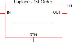
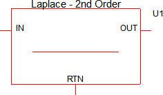
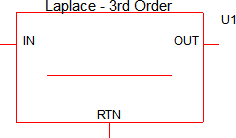
These filters are available in 1st, 2nd, and 3rd order versions and higher order filters can be realized by cascading two or more filters.
In this topic:
| Model Name: | Laplace Filters | ||||
| Simulator: | This device is compatible with the SIMPLIS simulator. | ||||
| Parts Selector Menu Locations: |
|
||||
| Symbol Library: | simplis_analog_functions.sxslb | ||||
| Model File: | simplis_analog_functions.lb | ||||
| Subcircuit Names: |
|
||||
| Symbols: |
|
||||
| Multiple Selections: | Multiple devices can be selected and edited simultaneously. | ||||
Editing the Laplace Filter
To configure the Laplace Filter, follow these steps:
- Double click the symbol on the schematic to open the editing dialog.
- Make the appropriate changes to the fields described in the table below the image.
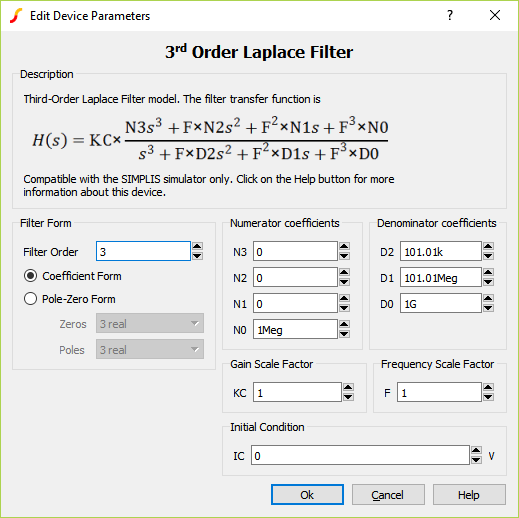
| Parameter Label | Units | Description |
| Filter Form - Filter Order | Desired filter order | |
| Numerator coefficient - N3 | Value of Numerator coefficient, N3 | |
| Numerator coefficient - N2 | Value of Numerator coefficient, N2 | |
| Numerator coefficient - N1 | Value of Numerator coefficient, N1 | |
| Numerator coefficient - N0 | Value of Numerator coefficient, N0 | |
| Denominator coefficient - D2 | Value of Denominator coefficient, D2 | |
| Denominator coefficient - D1 | Value of Denominator coefficient, D1 | |
| Denominator coefficient - D0 | Value of Denominator coefficient, D0 | |
| Gain Scale Factor - KC | Multiplier for gain | |
| Frequency Scale Factor - F | Multiplier for frequency. By setting this to {2*pi}, the radian frequencies will be transformed into Hertz. | |
| Initial Condition - IC | V | Initial output voltage of the device |
Transfer Function Form
One of the new features added to the Laplace filters in version 8.10 is the ability to enter the desired transfer function in Pole-Zero Form. In versions prior to 8.10, the transfer function could only be entered in coefficient form. You can select the desired entry form with the Filter Form radio buttons.
Pole-Zero Form
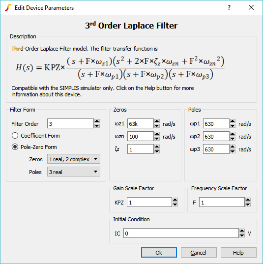
| Parameter Label | Units | Description |
| Filter Form - Filter Order | Desired filter order | |
| Filter Form - Zeros | Desired number of Zeros (real and complex) | |
| Filter Form - Poles | Desired number of Poles (real and complex) | |
| Zeros - ωz1 | rad/s | Desired zero location |
| Zeros - ωz2 | rad/s | Desired zero location |
| Zeros - ωz3 | rad/s | Desired zero location |
| Zeros - ωzn | rad/s | Natural undamped frequency |
| Zeros - ζz | Damping Ratio | |
| Poles - ωp1 | rad/s | Desired pole location |
| Poles - ωp2 | rad/s | Desired pole location |
| Poles - ωp3 | rad/s | Desired pole location |
| Zeros - ωpn | rad/s | Natural undamped frequency |
| Zeros - ζp | Damping Ratio | |
| Gain Scale Factor - KPZ | Multiplier for gain | |
| Frequency Scale Factor - F | Multiplier for frequency. By setting this to {2*pi}, the radian frequencies will be transformed into Hertz. | |
| Initial Condition - IC | V | Initial output voltage of the device |
Previous Version Compatibility
Beginning with version 8.10, an enhanced editing dialog was added allowing the transfer function to be defined in either coefficient or pole-zero form. The electrical model for the Laplace filters is unchanged from earlier versions. When using the Pole-Zero form, the dialog will calculate the coefficient form numerator and denominator values and write these values to the symbol. This calculation is performed after the dialog is closed, not after each pole or zero location is edited. This, in turn, preserves reverse compatibility with versions prior to Version 8.1. While the model will simulate in versions prior to Version 8.1, only the Coefficient Form dialog will appear and be editable. Likewise, Laplace filters placed in versions prior to 8.10 are compatible with 8.10 and future versions, both in terms of simulation and parameter editing dialogs.
Examples
Below are three examples of varying complexity which demonstrate how to use the Laplace filters.
Example - Simple 1st Order
The test circuit used to generate the waveform examples in the next section can be downloaded here: simplis_078_1st_order_laplace_example.sxsch.
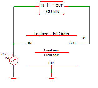
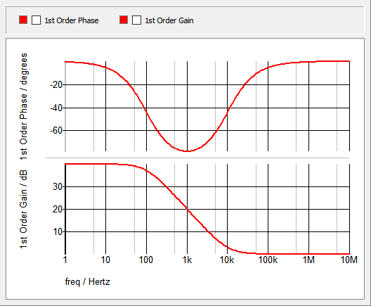
Waveforms - Simple 1st Order
This example uses a 1st order Laplace filter to implement a pole-zero transfer function. By setting the frequency scale factor equal to {2*pi} and using the Pole-Zero Form, the parameter entries are in Hertz and a single real pole is placed at 100Hz and a single real zero at 10kHz.
Example - 1st Order Low Pass Filter (LPF)
The test circuit used to generate the waveform examples in the next section can be downloaded here: simplis_078_1st_order_laplace_lpf_example.sxsch.
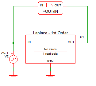
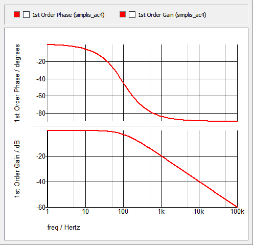
Waveforms - 1st Order Low Pass Filter (LPF)
This example uses a 1st order Laplace filter to implement a single pole filter with a 100Hz frequency. Using the Pole-Zero Form, a single real pole is placed at 100Hz and no zeros are used. Also, to have a 0dB DC gain, the Gain Scale Factor is adjusted. To set the DC gain to 0dB, the transfer function is solved for "KPZ" when "S=0" and "H(s)=1", the resulting Gain Scale Factor, KPZ is {2*pi*100}.
Example - Buck Converter 3rd Order Compensation
The test circuit used to generate the waveform examples in the next section can be downloaded here: simplis_078_buck_converter_3_order_compensation.sxsch
In this example, a synchronous buck converter is used to compare an OpAmp with type III compensation to a Laplace filter equivalent. The type III compensator is shown below, and the values for the resistors and capacitors are defined in the F11 window of the schematic:
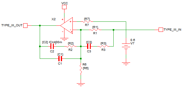
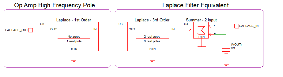
Since the typical type III compensator uses 2 zeros and 3 poles, the resistors, capacitors, and OpAmp are replaced with a 3rd order Laplace filter with 2 real zeros and 3 real poles. The OpAmp in this example is not ideal - it has a high frequency pole. An additional 1st order Laplace filter with 1 real pole at 700kHz and no zeros is used to model the high frequency behavior of the OpAmp. The equivalent filter schematic is shown below:
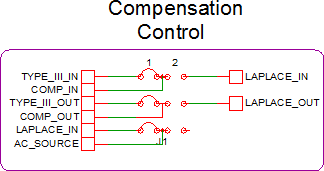
This example uses a set of jumpers to allow you to change between using the original type III compensator and the Laplace filter compensator. Select jumper position 1 to use the type III compensator and select jumper position 2 to use the Laplace filter compensator:
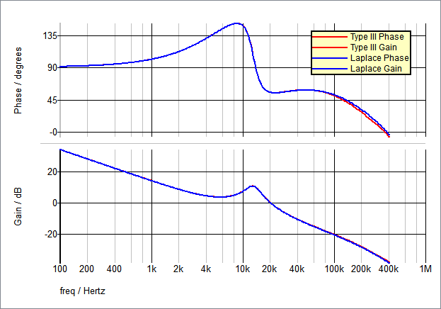
Waveforms - Buck Converter 3rd Order Compensation
The image below is derived from two separate simulation runs where the closed loop gain and phase waveforms of the Laplace filter simulation results were superimposed over the Type III compensator simulation results. Slight variations are due to the fact that the Op Amp is not ideal.