Random Probes
In this topic:
General Behaviour
A wide range of functions are available from the schematic Probe and Probe AC/Noise menus. With a few exceptions detailed below, all random probe functions have the following behaviour.
- If there are no graph windows open, one will be created.
- If a graph window is open and the currently displayed sheet has a compatible x-axis to what you are probing, the new curve will be added to that sheet. E.g. if the currently displayed graph is from a transient analysis and has an x-axis of Time, and you are also probing the results of a transient analysis, then the new curve will be added to the displayed graph. If, however the displayed curve was from an AC analysis, its x-axis would be frequency which is incompatible. In this case a new graph sheet will be created for the new curve.
will always create a new graph.
Functions
The following table shows all available random probe functions. Many of these can be found in the schematic's Probe menu while others are only available from
| Function |
| Single Ended Voltage |
| Single Ended Voltage - AC coupled |
| Single Ended Voltage - dB |
| Single Ended Voltage - Phase |
| Single Ended Voltage - Fourier |
| Single Ended Voltage - Nyquist |
| Single Ended Voltage - Normalised dB |
| Single Ended Voltage - Group delay |
| Differential Voltage |
| Differential Voltage - dB |
| Differential Voltage - Phase |
| Differential Voltage - Fourier |
| Differential Voltage - Nyquist |
| Differential Voltage - Normalised dB |
| Differential Voltage - Group delay |
| Relative Voltage - dB |
| Relative Voltage - Phase |
| Relative Voltage - Nyquist |
| Relative Voltage - Normalised dB |
| Relative Voltage - Group delay |
| Single Ended Current - In device pin |
| Single Ended Current - AC coupled in device pin |
| Single Ended Current - In wire |
| Single Ended Current - dB |
| Single Ended Current - Phase |
| Single Ended Current - Fourier |
| Single Ended Current - Nyquist |
| Single Ended Current - Normalised dB |
| Single Ended Current - Group delay |
| Differential Current - Actual |
| Differential Current - dB |
| Differential Current - Phase |
| Differential Current - Fourier |
| Differential Current - Nyquist |
| Differential Current - Normalised dB |
| Differential Current - Group delay |
| Power |
| Impedance |
| Output noise (noise analysis only) |
| Input noise (noise analysis only) |
| Device noise (noise analysis only) |
| Arbitrary expressions and XY plots |
Notes on Probe Functions
Impedance
You may plot the AC impedance at a circuit node using .This only works in AC analysis. This works by calculating V/I at the device pin selected.
Device Power
Device power is available from . This works by calculating the sum of VI products at each pin of the device. Power is not stored during the simulation. However, once you have plotted the power in a device once, the result is stored with the vector name:
device_name#pwr
E.g. if you plot the power in a resistor R3, its power vector will be called R3#pwr. You can use this as part of an expression in any future plot.
Note that, because SIMetrix is able to find the current in a sub-circuit device or hierarchical block, it can also calculate such a device's power. Be aware, however, that as this power is calculated from the VI product of the device's pins, the calculation may be inaccurate if the sub-circuit uses global nodes.
Plotting Noise Analysis Results
Small signal noise analysis does not produce voltage and current values at nodes and in devices in the way that AC, DC and transient analyses do. Noise analysis calculates the overall noise at a single point and the contribution of every noisy device to that output noise. Optionally the input referred noise may also be available.
To Plot Output Noise
- Select menu
To Plot Input Referred Noise
- Select menu
To Plot Device Noise
- Select menu
- Click on device of interest
Plotting Transfer Function Analysis Results
No cross-probing is available with transfer function analysis. Instead, you must use the general purpose Define Curve dialog box. With this approach you must select a vector name from a list. Proceed as follows:
- Select menu
- Select a value from the Available Vectors drop down box.
Transfer Function Vector Names
The vector names for transfer function will be of the form:
- source_name#Vgain
- source_name#Transconductance
- source_name#Transresistance
- source_name#Igain
where source_name is the name of a voltage or current source.
The vectors Zout, Yout or Zin may also be available. These represent output impedance, output admittance and input impedance respectively.
For more information see the Command Reference/.TF chapter of the Simulator Reference Manual.
Fourier Analysis
A Fourier spectrum of a signal can be obtained in a number of ways. You have a choice of using the default settings for the calculation of the Fourier spectrum or you can customise the settings for each plot. The following menus use the default settings:
- Graph menu:
- Graph menu:
Default Settings
The default fourier spectrum settings are:
| Setting | Default value |
| Method | Interpolated FFT |
| Number of points | Next integral power of two larger than number of points in signal |
| Interpolation order | 2 |
| Span | All data except which uses cursor span |
Custom Settings
With menu you will see the dialog below. With the menus a dialog box similar to that shown in Plotting an Arbitrary Expression will be displayed but will include a Fourier tab. Click on the this tab to display the Fourier analysis options as shown below.
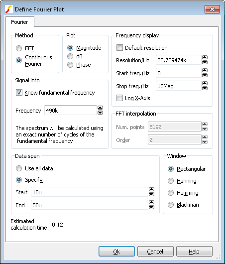
Method
SIMetrix offers two alternative methods to calculate the Fourier spectrum: FFT and Continuous Fourier.
The simple rule is: use FFT unless the signal being examined has very large high frequency components as would be the case for narrow sharp pulses. When using Continuous Fourier, keep an eye on the Estimated calculation time shown at the bottom right of the dialog.
A description of the two techniques and their pros and cons follows.
| FFT | Fast Fourier Transform. This is an efficient algorithm for calculating a discrete Fourier transform or DFT. DFTs generally operate on evenly spaced sampled data. Unfortunately the data generated by the simulator is not evenly spaced so it is therefore necessary to interpolate the data before presenting it to an FFT algorithm. The interpolation process is in effect the sampling process and the Nyquist sampling theorem applies. This states that the signal can be perfectly reproduced from the sampled data if the sampling rate is greater than twice the maximum frequency component in the signal. In practice this condition can never be met perfectly and any signal components whose frequency is greater than half the sampling rate will be aliased to a different frequency. So if the number of interpolated points is too small there will be errors in the result due to high frequency components being aliased to lower frequencies. This is the Achilles heel of FFTs applied to simulated data. The Continuous Fourier technique, described next, does not suffer from this problem. It suffers from other problems the main one being that it is considerably slower than the FFT. |
| Continuous Fourier | This calculates the Fourier spectrum by numerically integrating the Fourier integral. With this method, each frequency component is calculated individually whereas with the FFT the whole spectrum is calculated in one - quite efficient - operation. Continuous Fourier does not require the data to be interpolated and does not suffer from aliasing. The problem with continuous Fourier is that compared to the FFT it is a slow algorithm and in many cases an FFT with a very large number of interpolated points can be calculated more quickly and give just as accurate a result. However, in cases where a signal has a very large high frequency content - such as narrow pulses - this method is superior and it is recommended that it is used in preference to the FFT in such situations. The continuous Fourier technique has the additional advantage that it can be applied with greater confidence as the aliasing errors will not be present. It does have its own source of error due to the fact that simulated data itself is not truly continuous but represented by unevenly spaced points with no information about what lies between the points. This error can be minimised by ensuring that close simulation tolerances are used. See Simulator Reference Manual/Convergence, Accuracy and Performance for details. Because each frequency component is calculated individually, the calculation time is affected by the values entered in Frequency Display. |
Plot (Phase or Magnitude)
The default is to plot the magnitude of the Fourier spectrum. Select Phase if you require a plot of phase or dB if you need the magnitude in dBs.
Frequency Display
| Resolution/Hz | Available only for the continuous Fourier method. This is the frequency interval at which the spectral components are evaluated. It cannot be less than 1/T where T is the time interval over which the spectrum is calculated. |
| Start Freq./Hz | Start frequency of the display. |
| Stop Freq./Hz | Stop frequency of the display. |
| Log X-Axis | Check this to specify a logarithmic x-axis. This will force a minimum value for the start frequency equal to 1/T where T is the time interval being analysed. |
Signal Info
If the signal being analysed is repetitive and the frequency of that signal is known exactly then a much better result can be obtained if it is specified here. Check the Know fundamental frequency box then enter the frequency. The Fourier spectrum will be calculated using an integral number of complete cycles of the fundamental frequency. This substantially reduces spectral leakage. Spectral leakage occurs because both the Fourier algorithms work on an assumption that the signal being analysed is a repetition of the analysed time interval from ???MATH???t=-\infty???MATH??? to ???MATH???t=+\infty???MATH???. If the analysed time interval does not contain a whole number of cycles of the fundamental frequency this will be a poor approximation and the spectrum will be in error. In practice this problem is minimised by using a window function applied to the signal prior to the Fourier calculation, but using a whole number of cycles reduces the problem further.
Note that the fundamental frequency is not necessarily the lowest frequency in the circuit but the largest frequency for which all frequencies in the circuit are integral harmonics. For example if you had two sine wave generators of 1kHz and 1.1KHz, the fundamental is 100Hz, not 1kHz; 1kHz is the tenth harmonic, 1.1KHz is the eleventh.
You should not specify a fundamental frequency for circuits that have self-oscillating elements.
FFT Interpolation
As explained above, the FFT method must interpolate the signal prior to the FFT computation. Specify here the number of points and the order. The number of points entry may be forced to a minimum if a high stop frequency is specified in the Frequency Display section.
The number of interpolation points required depends on the highest significant frequency component in the signal being analysed. If you have an idea what this is, a useful trick to set the number of points to a suitable value, is to increase the stop frequency value in the Frequency Display section up to that frequency. This will automatically set the number of interpolation points to the required value to handle that frequency. If you don't actually want to display frequencies up to that level, you can bring the stop frequency back down again. The number of interpolation points will stay at the value reached.
If in doubt, plot the FFT twice using a different number of points. If the two results are significantly different in the frequency band of interest, then you should increase the number of points further.
Usually an interpolation order of 2 is a suitable value but you should reduce this to 1 if analysing signals with abrupt edges. If analysing a smooth signal such as a sinusoid, useful improvements can be gained by increasing the order to 3.
Advanced Options
Pressing the Advanced Options...
button will open this dialog box:
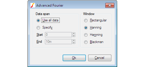
Data Span
Usually the entire simulated time span is used for the fourier analysis. To specify a smaller time interval click Specify and enter the start and end times.
Note that if you specify a fundamental frequency, the time may be modified so that a whole number of cycles is used. This will occur whether or not you explicitly specify an interval.
Window
A window function is applied to the time domain signal to minimise spectral leakage (See above).
The choice of window is a compromise. The trade off is between the bandwidth of the main spectral component or lobe and the amplitude of the side-lobes. The rectangular window - which is in effect no window - has the narrowest main lobe but substantial side-lobes. The Blackman window has the widest main lobe and the smallest side lobes. Hanning and Hamming are something in between and have similar main lobe widths but the side lobes differ in the way they fall away further from the main lobe. Hamming starts smaller but doesn't decay whereas Hanning while starting off larger than Hamming, decays as the frequency moves away from the central lobe.
Despite the great deal of research that has been completed on window functions, for many applications the difference between Hanning, Hamming and Blackman is not important and usually Hanning is a good compromise.
There are situations where a rectangular window can give significantly superior results. This requires that the fundamental frequency is specified and also that the simulated signal is consistent over a large number of cycles. The rectangular window, however, usually gives considerably poorer results and must be used with caution.
Probing Buses
It is possible to probe a bus in which case a plot representing all the signals on the bus will be created. Usually this will be a numeric display of the digital bus data, but it is also possible to display the data as an analog waveform. Buses may contain either digital or analog signals; if any analog signals are present then threshold values must be supplied to define the logic levels of the analog signals.
To probe bus using default settings
Use the schematic popup menu Probe Voltage... or hot key F4 and probe the bus in the same way as you would a single wire.
This will plot a numeric trace using decimal values.
To probe bus using custom settings
- Select menu
- Click on desired bus.
- Enter the desired bus parameters as described in Bus Probe Options.
Bus Probe Options
The following describes the options available for random and fixed bus probes. These options are set using the dialog box shown below. See Probing Buses and Fixed Probe Options for details on plotting buses.
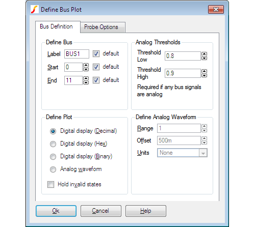
Define Bus
| Label | This is how the curve will be labelled in the plot |
| Start, End | Defines which wires in the bus are used to created the displayed data. The default is to use all wires. |
Plot Type
| Decimal/Hexadecimal/Binary | Each of these specifies a numeric display (see below) showing the bus values in the number base selected. |
| Analog waveform | Specifies that the bus data should be plotted as an analog waveform. |
| Hold invalid states | If checked, then and invalid digital states found in the data will be replaced with the most recent valid state. If not checked, invalid states will be shown as an 'X' in numeric displays. This option is automatically selected for analog waveform mode. |
Analog Thresholds
These are required if any of the signals on the bus is analog. These define the thresholds for converting to logic levels.
| Threshold | Low Analog voltage below which the signal is considered a logic zero. |
| Threshold | High Analog voltage above which the signal is considered a logic one. |
If a signal is above the lower threshold but below the upper threshold, it will be considered as 'unknown'.
Define Analog Waveform
Only enabled if Analog waveform is specified in the Plot Type box. Specifies the scaling values and units for analog waveforms:
| Range | Peak-peak value used for display. |
| Offset | Analog display offset. A value of zero will result in an analog display centred about the x-axis. |
| Units | Select an appropriate unit from the drop down box. |
Plotting an Arbitrary Expression
If what you wish to plot is not in one of the probe menus, SIMetrix has a facility to plot an arbitrary expression of node voltages or device currents. This is accessed via one of the menus . Selecting one of these menus brings up the Define Curve dialog box shown below.
Define Curve Sheet
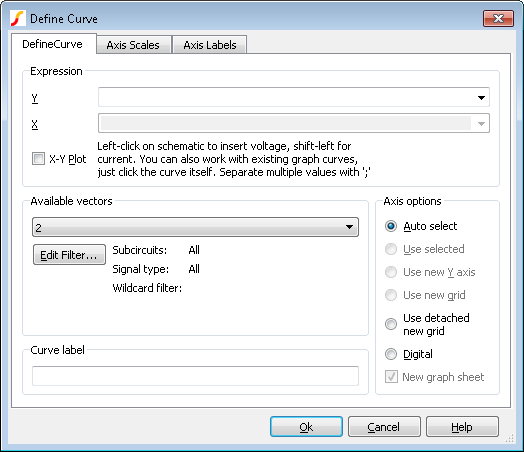
Expression
| Y | Enter arithmetic expression. This can use operators + - * / and \^ and various functions such as log, sin etc. To enter a node voltage, click on a point on the schematic. To enter a device pin current, hold down the shift key and click on the device pin in the schematic. Both voltages and currents may also be selected from the Available Vectors box. You may also plot an expression based on any curve that is already plotted. Simply click on the curve itself and you should see a function entered in the form cv(n) where n is some integer. Any entries made in this box are stored for future retrieval. Use the drop down box to select a previous entry. |
| X | Expression for X data. Only required for X-Y plot and you must check X-Y Plot box. Expression entered in the same way as for Y data. |
Available Vectors
Lists values available for plotting. This is for finding vectors that aren't on a schematic either because the simulation was made direct from a netlist or because the vector is for a voltage or current in a sub-circuit. Refer to Data Handling and Keeps for more information. Press Edit Filter to alter selection that is displayed. See below.
The names displayed are the names of the vectors created by the simulator. The names of node voltages are the same as the names of the nodes themselves. The names for device currents are composed of device name followed by a '#' followed by the pin name. Note that some devices output internal node voltages which could get confused with pin currents. E.g. q1#base is the internal base voltage of q1 not the base current. The base current would be q1#b. For the vector names output by a noise analysis refer to Simulator Reference Manual/Command Reference/.NOISE.
Edit Filter...
Pressing the Edit Filter...
button opens:
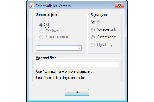
This allows you to select what is displayed in the available vectors dialog. This is useful when simulating large circuits and the number of vectors is very large.
Sub-circuit Filter
| All | Vectors at all levels are displayed. |
| Top level | Only vectors for the top-level are displayed |
| Select sub-circuit | All sub-circuit references will be displayed in the list box. Select one of these. Only vectors local to that sub-circuit will be displayed in Available Vector list. |
Signal Type
| All | List all signal types |
| Voltages Only | Only voltages will be listed |
| Currents Only | Only currents will be listed |
| Digital Only | Only digital vectors will be listed |
Wildcard filter
Enter a character string containing '*' and/or '?' to filter vector names. '*' matches 1 or more occurrences of any character and '?' matches any single character. Some examples:
| * | matches anything |
| X1.* | matches any signal name that starts with the three letters: X1. |
| X?.* | matches any name that starts with an X and with a '.' for the third letter. |
| *.q10#c | matches any name ending with .q10#c i.e the current into any transistor called q10 |
| *.U1.vout | matches any name ending with .U1.C11 i.e any node called vout in a subcircuit with reference U1. |
Curve Label
Enter text string to label curve
Axis Options
| Auto select | Select an appropriate axis automatically. See AutoAxis Feature |
| Use selected | Use currently selected y-axis |
| Use new Y-axis | Create a new y-axis in the selected grid. If there is more than one grid, the selected grid will have a double vertical line drawn at the far left. A grid can be selected by clicking in it |
| Use new Grid | Plots the curve in a new grid |
| Use detached new grid | Plots the curve in a new grid with a detached x-axis. A detached x-axis is independent and may be zoomed independently of other axes |
| Digital | Create a new digital axis. Digital axes are placed at the top of the window and are stacked. Each one may only take a single curve. As their name suggests, they are intended for digital traces but can be used for analog signals if required |
| New graph sheet | Creates a completely new graph sheet for the plot |
Note that you can move a curve to a new axis or grid after it has been plotted. See Moving Curves to Different Axis of Grid.
Axis Scales Sheet
Allows you to specify limits for x and y axes.
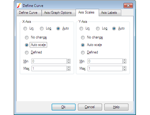
X-Axis/Y-Axis
| Lin/Log/Auto | Specify whether you want X-Axis to be linear or logarithmic. If Auto is selected, the axis (X or Y) will be set to log if the x values are logarithmically spaced. For the Y-axis it is also necessary that the curve values are positive for a log axis to be selected. |
| No Change | Keep axes how they are. Only relevant if adding to an existing graph. |
| Auto scale | Set limits to fit curves. |
| Defined | Set to limits defined in Min and Max boxes. |
Axis Labels Sheet
This sheet has four edit boxes allowing you to specify, x and y axis labels as well as their units. If any box is left blank, a default value will be used or will remain unchanged if the axis already has a defined label.
Curve Arithmetic
SIMetrix provides facilities for performing arithmetic on existing curves. For example you can plot the difference between two plotted curves.
-
With the menus:
- Plot | Sum Two Curves...
- Plot | Subtract Two Curves...
- Plot | Multiply Two Curves...
- Using the Add Curve... dialog box. With this method, select menu or then enter an expression as desired. To access an existing curve's data, simply click on the curve. For more information, see Plotting an Arbitrary Expression.
AC Analysis Notes on Curve Arithmetic
In AC analysis, the results are complex. When plotting a curve from an AC analysis, the magnitude of the complex data is plotted unless some other explicit function is applied such as phase() or imag(). Although the magnitude of the data is plotted, the graph system retains the original complex values. So any arithmetic operation performed directly on complex plotted data will also be complex. For example, if you have two curves from an AC analysis and you choose the Plot | Subtract Two Curves... menu to subtract them, the new result will be the magnitude of the complex difference not the difference in the magnitudes as might be expected. In mathematical terms, you will see |a-b| not |a|-|b|.
Using Random Probes in Hierarchical Designs
Random probes may successfully be employed in hierarchical designs. There are however some complications that arise and these are explained below.
Closed Schematics
Read the following if you find situations where cross-probing inside hierarchical blocks sometimes fails to function.
The names used for cross-probing are stored in the schematic itself and are saved to the schematic file. These netnames are not assigned until the netlist is created and this doesn't usually happen until a simulation is run. A problem arises, however, if the schematic is not open. If netnames have never been created then they won't be updated during the run as, by default, SIMetrix will not update a closed file.
This problem can be resolved by giving SIMetrix permission to update schematic files that are closed. To do this, type at the command line:
Set UpdateClosedSchematics
This only needs to be done once. Note that you can only do this with the full versions of SIMetrix.
This problem won't arise if you always run every schematic at least once while it is open. If you do this, the netnames will be updated and you will be prompted to save the schematic before closing it.
Multiple Instances
An issue arises in the situation where there are multiple instances of a block attached to the same schematic. Consider the following top level circuit.
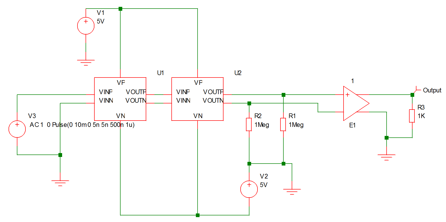
This has two instances of the block fastamp.sxsch U1 and U2. Suppose you wanted to plot the voltage of a node inside U1. The schematic fastamp.sxsch is open but to which block does it refer? The answer is that it will refer to the most recent block that was used to descend into it. The block that a schematic refers to is always displayed in the schematic's status bar as illustrated below
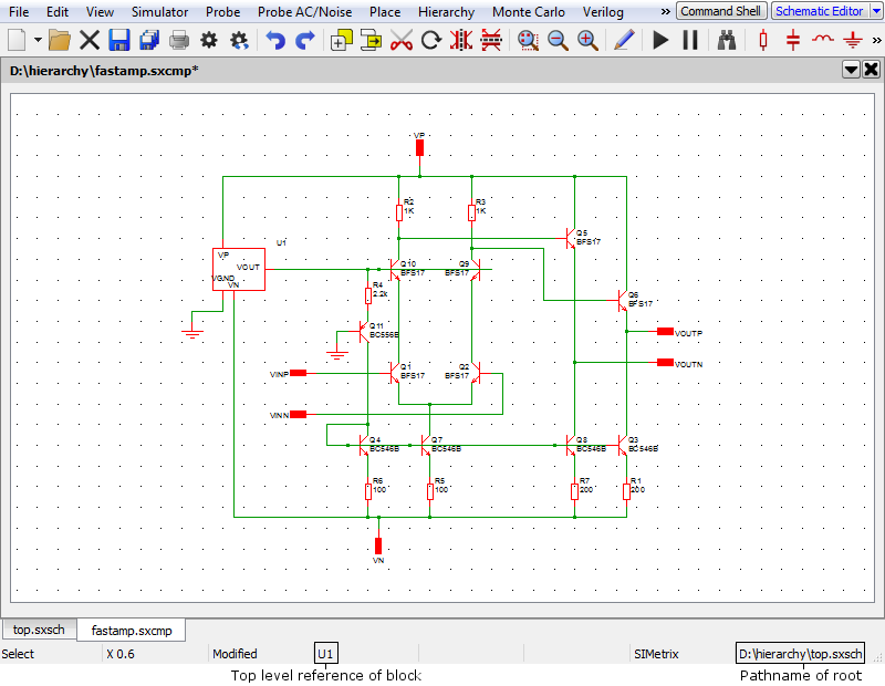
To plot a node in U2, ascend to parent (top.sxsch in the above example) then descend into U2. The same schematic as above will be displayed but will now refer to U2 instead of U1.
Plotting Currents
In the same way that you can plot currents into subcircuits in a single sheet design, so you can also plot currents into hierarchical blocks at any level.
Plotting the Results from a Previous Simulation
-
Select the menu item . This will open a dialog box similar to the following:
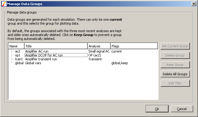
- Select the name of the previous run (or group) that you require. The current group will be highlighted. Note that the AC analysis mode generates two groups. One for the AC results and the other for the dc operating point results. Transient analysis will do the same if the start time is non-zero. The names for the groups usually default to the file name of the schematic that generated them. (They have been edited to be more meaningful in the picture above).
- Click Set Current Group
- Click Ok
- Plot the result you require in the normal way. A word of warning: If the schematic has undergone any modifications other than part value changes since the old simulation was completed, some of the netnames may be different and the result plotted may not be of what you were expecting.
| Note |
By default, only the three most recent groups are kept. This can be changed using the GroupPersistence option using the Set command - see Set). You can also keep specify that a particular group is kept permanently using the Data Groups Manager. Proceed as follows:
|
Combining Results from Different Runs
There are occasions when you wish to - say - plot the difference between a node voltage for different runs. You can do this in SIMetrix using the menu by entering an expression such as 'vector1 -vector2 ' in the y-expression box, where vector1 and vector2 are the names of the signals. However, as the two signals come from different runs we need a method of identifying the run. This is done by prefixing the name with the group name followed by a colon. The group name is an analysis type name (tran, ac, op, dc, noise, tf or sens) followed by a number. The signal name can be obtained from the schematic. For voltages, move the cursor over the node of interest and you will see the name appear in the status box in the form "NET=???". For currents put the cursor on a device pin and press control-P. The group name is displayed in the simulator progress box when the simulation is running. You can also find the current group by selecting menu . The current group is marked current in the Flags column.
Here is an example. In tutorial 1, the signal marked with the Amplifier Output probe is actually called Q3_E. The latest run (group) is called tran4. We want to plot the output subtracted from the output for the previous run. The previous run will be tran3. So we enter in the y-expression box:
tran4:q3_e-tran3:q3_e
For more details on data groups, please refer to the Script Reference Manual/Script Language/Accessing Simulation Data.
| ◄ Fixed Probes | Plot Journals and Updating Curves ▶ |