5.4 Exploiting the Netlist Preprocessor
To download the examples for Module 5, click Module_5_Examples.zip.
In this topic:
The netlist preprocessor was introduced in the 3.0.1 What Happens When You Press F9? topic. This introductory topic gave an overview of the netlist preprocessor from the point of view of running a model. This topic focuses on creating models, and how to use the netlist preprocessor to make the model more robust and often, easier to construct.
What You Will Learn
When the netlist preprocessor is invoked and which subcircuits it modifies, and using the netlist preprocessor, you can:
- Create and change the value of variables using the .VAR statement.
- Define conditional statements with the .IF/.ELSE/.ENDIF construct.
- Test for the existence of variables
- Create "Case" statements, where a set of variables are created based on "case" variable.
- Output comments to the simulation deck file for debugging.
- Determine the currently executing SIMPLIS analyses. The model can then be configured based on the analysis types.
- Abort the simulation with the .ERROR statement, typically this is placed inside a .IF statement.
- Loop with the .WHILE construct.
Getting Started
The netlist preprocessor is called whenever you run a SIMPLIS simulation. During the run process described in 3.0.1 What Happens When You Press F9?, the netlist file is created from the schematic and the contents of the F11 window are placed at the top of the netlist file. This file is then passed through the netlist preprocessor to create a deck file. This deck file is the file which SIMPLIS uses to run the simulation. Because the netlist preprocessor is called on the netlist, including the F11 window contents, the language described in this topic applies equally to the F11 window text or to a subcircuit model. The subcircuit model could be defined in a model file or directly in the F11 window.
- Assign variables, both as scalars (a single value) and vectors (a collection of values).
- Test for the existence of variables
- Conditionally branch (if-else logic)
- Loop
The netlist preprocessor differs from a general purpose programming language in the task at hand - the netlist preprocessor is designed with a single minded goal: to create a text model for use in the SIMetrix or SIMPLIS simulators. Because of this goal, the output of the netlist preprocessor is a simple chunk of text which represents a model. For review, a practical example taken from 3.0.2 What Actual Device is Simulated in SIMPLIS?, will be discussed next.
Subcircuit Creation Slideshow
The following slideshow shows the netlist preprocessor as it steps through the model definition from the library, and generates the actual subcircuit. Note that the netlist preprocessor eliminates any blank lines and all comment lines which begin with an asterisk.
- You can pause the slideshow by moving the mouse cursor over the images.
- To go forward or back one slide, click the arrow links that appear when you mouse over the slideshow. You can also use the left and right arrow keys to go forward or to go back one slide.
- You can jump to a particular slide by clicking one of the gray squares at the bottom on the image. The current slide is indicated by the white square.
- Parameters passed into the subcircuit on the netlist instantiation line
- Conditional if-else statements
- Variables defined with the .VAR statement
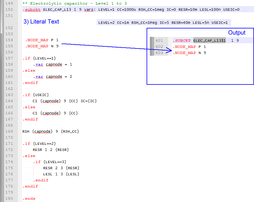
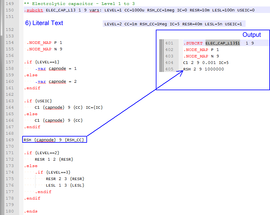
- Literal text from the input file
Invoking the Preprocessor
X$C1 17 0 ELEC_CAP_L13 vars: LEVEL=2 CC={1m*Gauss(0.20)} RSH_CC=1Meg IC=5 RESR=40m LESL=5n USEIC=1
Notice
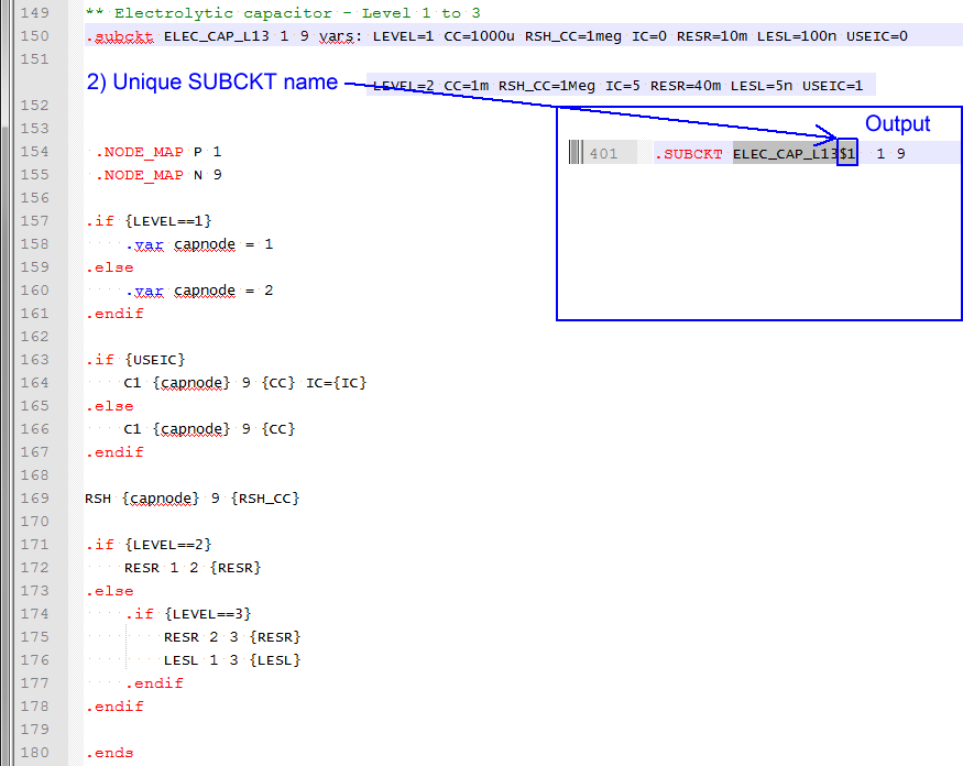
the vars: keyword on the netlist instantiation line, this tells the program
to preprocess this subcircuit and create a new subcircuit with a unique subcircuit name
using the preprocessor. There are cases where a subcircuit is completely static and has no
parameters passed into it, and in this case, there is no vars: keyword on
the netlist instantiation line, and the preprocessor is not invoked.Creating Variables
Variables In The F11 Window
Creating variables in the F11 window is straightforward and was first discussed in the 3.0.1 What Happens When You Press F9? topic. You simply enter the variable name and value in a .VAR statement. For example, to create a Rload variable with a value of 2.5, the following syntax is used:
.var RLoad=2.5
This defines a variable RLoad with a value of 2.5. Once a variable is defined, you can use that variable in another variable statement, by enclosing the right hand side of the equal sign inside curly braces {}. For example:
.var VOUT=1.5
.var Iload=2.8
.var Rload={Vout/Iload}
The first two statements create VOUT and Iload variables and then calculate a Rload variable from the ratio of VOUT and Iload with a calculated value of 0.5357142857142857.
Case Sensitivity
Variables are NOT case sensitive. In the above example, the variable VOUT was created, and the variable Vout was used to calculate the value of the Rload variable. VOUT and Vout are the same variable and you don't need to worry about case sensitivity when creating or modifying variables.
The various "dot commands", such as .VAR are also not case sensitive, so .VAR is the same as .var.
Scope of F11 Window Variables
Each schematic or schematic component has it's own F11 window and variables entered into the F11 window are only available at that schematic level. You can define global variables using the .GLOBALVAR construct. For example, to create a VOUT variable which is available at every level of the hierarchy below the current level, use:
.GLOBALVAR VOUT=1.5
Global variables are not the preferred method of making variables available at multiple levels of hierarchy. A much better system uses the SIMPLIS_TEMPLATE property to pass the variables into the lower level of hierarchy. This was described in the 5.1 Passing Parameters into Subcircuits Using the SIMPLIS_TEMPLATE Property topic.
Creating Variables In a Subcircuit
Variables are defined in a subcircuit in the same way as in the F11 window. The difference is in the scope - variables defined in a subcircuit are only available in that subcircuit. Symbols on the top level or at other hierarchical levels cannot use these variables. Global variables defined in a subcircuit are available in that subcircuit and every hierarchical level below the subcircuit where the global variable is defined. Global variables defined in a subcircuit are not available for use on the top level, or other levels above the subcircuit where they are defined.
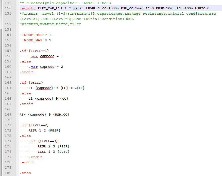
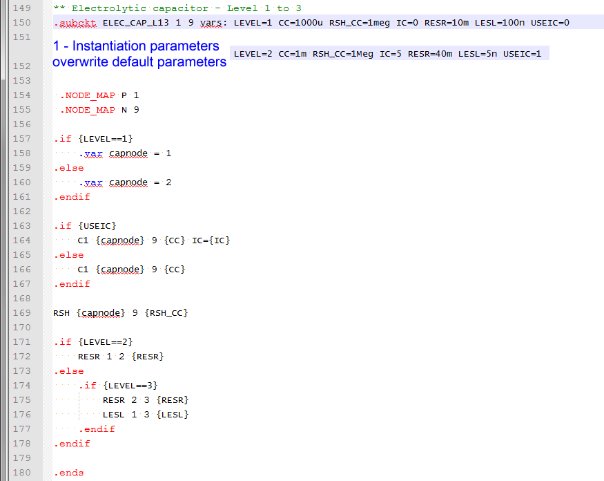
- The default parameters defined on the .subckt declaration line
- Parameters passed on the netlist instantiation line. Although these parameters usually have the same names as the parameters defined on the .subcircuit declaration line, you can also pass additional parameters and test for the existence of these parameters with the method described in the Testing For the Existence of Variables section.
- Global variables declared at a higher level of hierarchy
- Variables declared inside the subcircuit using the .VAR construct
.subckt ELEC_CAP_L13 1 9 vars: LEVEL=1 CC=1000u RSH_CC=1meg IC=0 RESR=10m LESL=100n USEIC=0
If no parameters were passed on the netlist instantiation line, these variables would be available in the subcircuit:
| Variable Name | Variable Value |
| LEVEL | 1 |
| CC | 1000u |
| RSH_CC | 1meg |
| IC | 0 |
| RESR | 10m |
| LESL | 100n |
| USEIC | 0 |
In the example instantiation line:
X$C1 17 0 ELEC_CAP_L13 vars: LEVEL=2 CC={1m*Gauss(0.20)} RSH_CC=1Meg IC=5 RESR=40m LESL=5n USEIC=1
each
variable is redefined and these instantiation line variables overwrite the values from the
subcircuit definition line. Variables, whether they are a single value, or a array of values, are defined with the .VAR statement. As mentioned above, parameters defined on the subcircuit definition line or passed into a subcircuit on the netlist instantiation line are automatically converted to variables inside the subcircuit. The next section describes several ways to create variables.
Creating Vectors
Vectors are created by enclosing the vector inside square brackets []. For example, the following syntax creates a vector of 4 elements, containing 0, 1, 2, and 3.
.var my_vec = {[0, 1, 2, 3]}
You can also use the built in vector Function, which creates a vector with each element value equal to the index. These two variable statements are functionally identical:
.var my_vec = {[0, 1, 2, 3]}
.var my_vec2 = {Vector(4)}
You can also create vectors from existing variables. For example, in SIMPLIS, PWL components are defined with a set of X-Y pairs. In the model definition for the Multi-Level PWL Capacitor w/ Level 0-3 (Version 8.0+), the X-Y pairs are passed into the model as scalar parameters, X0, X1, Y0, Y1, etc. In the model file, these scalar variables are collected into vectors, which are shown here in a shortened form:
.VAR exes = { [ X0, X1, X2, X3 ] }
.VAR eyes = { [ Y0, Y1, Y2, Y3 ] }
The model then uses a While Loop to create a PWL capacitor model from the exes and eyes vectors.
String Variables
String variables can be assigned by enclosing the string in single quotes:
.var my_string = '0_TO_1'
Testing For the Existence of Variables
You can always test for the existence of variables using the ExistVec Function, which returns true or false. You simply provide the variable name as a string to the function. A simple example which tests for the existence of a variable and creates the variable if it doesn't exist is as follows.
.IF { !ExistVec( 'VERSION' ) }
  .VAR VERSION = 2
.ENDIF
In the above logical test, the complement operator '!' is used to invert the ExistVec() function and thereby implement the pseudocode "if the VERSION vector doesn't exist, return true." The if branch is then entered and the VERSION variable is created.
Determining the Currently Executing Analyses
Starting with version 8.10, global variables are automatically created indicating the analysis types being executed. These variables are boolean (true/false) and are defined at the top level and can therefore be used at any level of the design hierarchy. In SIMPLIS mode, these variable names are:
- HAS_POP_ANALYSIS
- HAS_AC_ANALYSIS
- HAS_TRAN_ANALYSIS
An example using these global variables is located in the zip archive with schematic name: 5.9_has_analysis.sxsch. This example also uses the .IF/.ELSE conditional expression and the .ERROR statement.
Debugging
Debugging the model creation process can be difficult, as the nature of the preprocessor doesn't allow much in the way of interactive debugging. The only way to debug a model is to output comment statements to the actual model file. As these comments will be ignored by the SIMPLIS simulator, you can safely enter as many debug statements as required. To output a debug statement you use the following syntax:
{'*'} Comment here
The pseudocode for the above debug statement can be interpreted as "Evaluate a string '*', and output that to the file, followed by the literal text Comment here." More often than not, you will want to output a variable value as it was evaluated, for example the Rload value calculated in the above example:
.var VOUT=1.5
.var Iload=2.8
.var Rload={Vout/Iload}
{'*'} Value of Rload : {RLoad}
This example is located in the zip archive with schematic name: 5.10_debug_statement.sxsch.
You can open the deck file using the menu . The debug statement output in the deck file is:
* Value of Rload : 0.535714285714286
Branching With .IF/.ELSE/.ENDIF
The preprocessor allows branching using if-else logic. There is no elseif construct, you can either nest multiple if-else branches, or first test a variable to eliminate all invalid values, and then use multiple if-else constructs which are not nested. See The .ERROR Statement for an example of this.
The basic if-else logic syntax is as follows:
.IF { conditional expression }
statements to be executed if conditional expression is true
.ELSE
statements to be executed if conditional expression is false
.ENDIF
You can also omit the .ELSE portion of the if-else statement, which results in a simple if logic branch:
.IF { conditional expression }
statements to be executed if conditional expression is true
.ENDIF
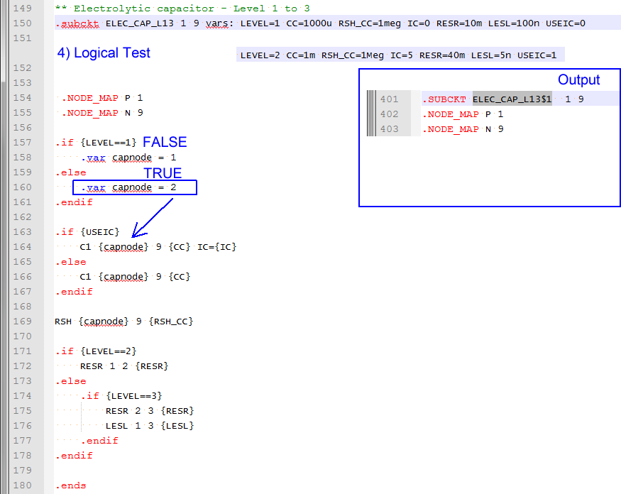
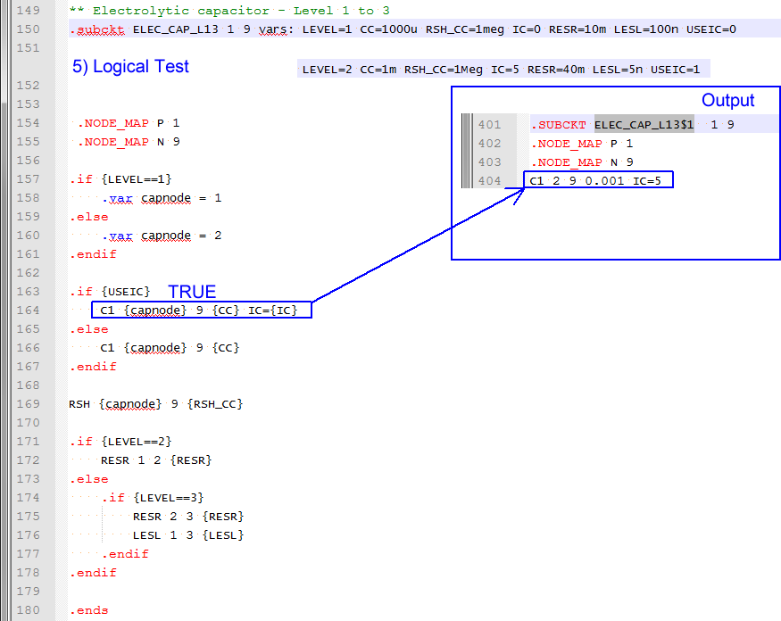
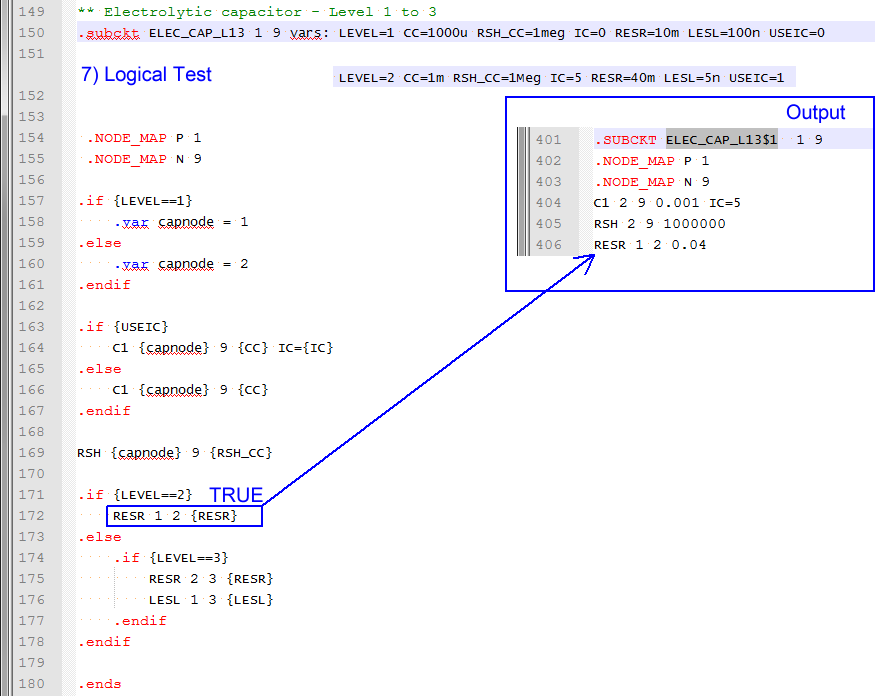
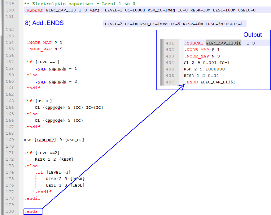
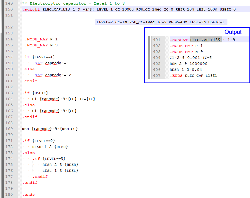
A practical example can be taken from the electrolytic capacitor example above. In that example, a variable is assigned a value based on the value of the LEVEL variable.
.if {LEVEL==1}
  .var capnode = 1
.else
  .var capnode = 2
.endif
The capnode variable was then used to create the connections between the capacitor and resistor (LEVEL=1) in the subcircuit. This is an important concept - variables which are created in a model can be used for any purpose, not just as component values for a particular instantiation, for example a resistance value. Assigning variables to represent node numbers allows you to literally build the schematic view of the model programatically. The Looping Using .WHILE/.ENDWHILE section is a very good example of this.
Nested Branching
The if-else construct can be nested, the syntax for this is:
.IF { conditional expression }
statements to be executed if conditional expression is true
.ELSE
  .IF { second conditional expression }
    statements to be executed if second conditional expression is true
  .ELSE
    statements to be executed if second conditional expression is false
  .ENDIF
.ENDIF
As you can see, as the number of nested if-else statements increases, the code becomes increasingly complex. In the next section, you will learn how to test variables to make sure the variables are within an allowed range. You will see that this eliminates the need for the nested if-else construct, and at the same time creates a more robust model.
The .ERROR Statement
Quite often, the conditional expressions used in if-else logic expects the parameters used in the conditional expressions to be within some known range. For this reason, the .ERROR statement has been added to the preprocessor and prevents the model from running if a parameter value is out of range. The way this works is very simple - if a .ERROR statement exists in the deck file output from the preprocessor, the simulation is halted and an error message is output. The best way to learn about the .ERROR statement is to examine a practical example. In this example, the VOUT variable is expected to take on one of two values, 1.0 or 1.2 volts. The inductance and capacitance values L_VALUE and C_VALUE are then calculated based on the VOUT value. This is a classic "case" or "switch" logic implementation.
This example is located in the zip archive with schematic name: 5.11_nested_if_else_statement.sxsch.
*** The master case or switch variable
.VAR VOUT=3.3

*** first, setup default values:
.VAR L_VALUE = 390n
.VAR C_VALUE = {4*22u}

*** use .IF/.ELSE branching to determine inductor/capacitor values
.IF { VOUT == 1.0 }
	.VAR L_VALUE = 390n
	.VAR C_VALUE = {8*22u}
.ELSE
	.IF { VOUT == 1.2 }
		.VAR L_VALUE = 470n
		.VAR C_VALUE = { 5*22u }
	.ENDIF
.ENDIF

*** debug
{ '***' } L_VALUE : { L_VALUE }
{ '***' } C_VALUE : { C_VALUE }
In the above text, the default values of L_VALUE and C_VALUE must be defined because it is possible that the VOUT variable will take on a value which is not 1.0 or 1.2. In fact, in the above example, the VOUT variable has been purposely set to a value which will result in the default values being used. A better solution would be to limit the acceptable values of the VOUT variable to values which are present in the nested if-else logic.
This example is located in the zip archive with schematic name: 5.12_error_and_nested_if_statements.sxsch.
*** The master case or switch variable
.VAR VOUT=3.3

.IF { VOUT != 1.0 && VOUT != 1.2 }
  .ERROR "Invalid VOUT parameter value. Acceptable values are 1.0 and 1.2, value is {VOUT}"
.ENDIF

*** first, setup default values:
.VAR L_VALUE = 390n
.VAR C_VALUE = {4*22u}

*** use .IF/.ELSE branching to determine inductor/capacitor values
.IF { VOUT == 1.0 }
	.VAR L_VALUE = 390n
	.VAR C_VALUE = {8*22u}
.ELSE
	.IF { VOUT == 1.2 }
		.VAR L_VALUE = 470n
		.VAR C_VALUE = { 5*22u }
	.ENDIF
.ENDIF

*** debug
{ '***' } L_VALUE : { L_VALUE }
{ '***' } C_VALUE : { C_VALUE }
When you run the above example, the following error message is output to the command shell:
*** ERROR *** (5.12_error_and_nested_if_statements.net;18):
Invalid VOUT parameter value. Acceptable values are 1.0 and 1.2, value is 3.3
A few new concepts are introduced in the above code snippet. Firstly, in the conditional expression:
.IF { VOUT != 1.0 && VOUT != 1.2 }
the "not equals to" logical operator is used. This is the two character sequence "!=", and is used twice to test the two values. There is a logical "and" operator (&&) used to logically "and" the results of the two "not equals to" operations. The second concept is the .ERROR syntax itself:
.ERROR "Invalid VOUT parameter value. Acceptable values are 1.0 and 1.2, value is {VOUT}"
While this is pretty straightforward, one comment needs to be made - the entire error message text must be enclosed in double quotes, as it contains space characters. Also the {VOUT} variable is evaluated and this capability to evaluate variables inside the .ERROR statement was added to version 8.00. Versions prior to 8.00 will output {VOUT} as literal text.
Now that the VOUT variable is limited to known good values, we can un-nest the if-else logic and eliminate the default values.
This example is located in the zip archive with schematic name: 5.13_error_and_unnested_if_statements.sxsch.
*** The master case or switch variable
.VAR VOUT=3.3

.IF { VOUT != 1.0 && VOUT != 1.2 }
  .ERROR "Invalid VOUT parameter value. Acceptable values are 1.0 and 1.2, value is {VOUT}"
.ENDIF

*** use .IF branching to determine inductor/capacitor values
.IF { VOUT == 1.0 }
	.VAR L_VALUE = 390n
	.VAR C_VALUE = {8*22u}
.ENDIF

.IF { VOUT == 1.2 }
	.VAR L_VALUE = 470n
	.VAR C_VALUE = { 5*22u }
.ENDIF

*** debug
{ '***' } L_VALUE : { L_VALUE }
{ '***' } C_VALUE : { C_VALUE }
When this example is simulated, the following error messages and warnings are output to the command shell:
*** ERROR *** (5.13_error_and_unnested_if_statements.net;18):
Invalid VOUT parameter value. Acceptable values are 1.0 and 1.2, value is 3.3
*** Warning *** (5.13_error_and_unnested_if_statements.net;34): Error : Cannot find vector of name 'C_VALUE'

*** Warning *** (5.13_error_and_unnested_if_statements.net;33): Error : Cannot find vector of name 'L_VALUE'
Using The Search Function In Conditional Expressions
In the above example, the VOUT variable was tested against two acceptable values in the following .IF statement
.IF { VOUT != 1.0 && VOUT != 1.2 }
You can see that, as the number of acceptable values increases, this conditional statement will become prohibitively long. Instead of using this "not equal to"/"and" logic to form the conditional expression, you can define the acceptable values as a vector and search that vector for the variable value. The Search Function returns the index into the vector where the match is found, or -1 if the test value doesn't exist in the vector. Using the Search function, the same conditional expression could be written as follows:
.IF { Search( [ 1.0, 1.2 ] , VOUT ) == -1 }
In pseudocode, this would read "Search the vector containing 1.0 and 1.2 for VOUT and if VOUT isn't found in the vector, return true."
The entire code snippet using Search logic would be as follows.
This example is located in the zip archive with schematic name: 5.14_error_using_search_function.sxsch.
*** The master case or switch variable
.VAR VOUT=3.3

.IF { Search( [ 1.0, 1.2 ] , VOUT ) == -1 }
  .ERROR "Invalid VOUT parameter value. Acceptable values are 1.0 and 1.2, value is {VOUT}"
.ENDIF

*** no need for .else branches because we have eliminated all invalid values.
*** use .IF branching to determine inductor/capacitor values
.IF { VOUT == 1.0 }
	.VAR L_VALUE = 390n
	.VAR C_VALUE = {8*22u}
.ENDIF

.IF { VOUT == 1.2 }
	.VAR L_VALUE = 470n
	.VAR C_VALUE = { 5*22u }
.ENDIF

*** debug
{ '***' } L_VALUE : { L_VALUE }
{ '***' } C_VALUE : { C_VALUE }
When this example is simulated, the following error messages and warnings are output to the command shell:
*** ERROR *** (5.14_error_using_search_function.net;18):
Invalid VOUT parameter value. Acceptable values are 1.0 and 1.2, value is 3.3
*** Warning *** (5.14_error_using_search_function.net;35): Error : Cannot find vector of name 'C_VALUE'

*** Warning *** (5.14_error_using_search_function.net;34): Error : Cannot find vector of name 'L_VALUE'
Looping Using .WHILE/.ENDWHILE
The netlist preprocessor implements a while loop with the .WHILE and .ENDWHILE construct. Although at first glance, while loops might seem inconvenient compared to a for loop, you can create any structured program with just a while loop and if-else construct.
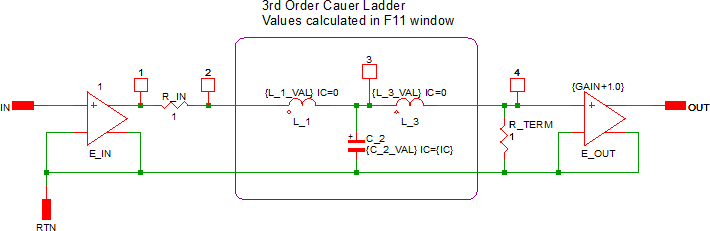
The capstone example in this topic is a Butterworth filter with programmable filter order, pole frequency, and gain, implemented with a Cauer ladder network. To create this filter using a schematic would be difficult as the actual schematic is not fixed and changes based on the filter order. As more poles are added, the cauer ladder size increases. You can think of the while loop as a way to programatically construct the equivalent schematic based on the input parameters. A schematic view of a third order Butterworth filter implemented with a cauer ladder is as follows:
Examples circuits which demonstrate the while loop are located in the zip archive with schematic names: 5.15_while_example_w_fixed_schematic.sxsch and 5.16_while_loop_example.sxsch.
The following preprocessor code snippet uses a cauer ladder to create a Butterworth filter with between 1 and 6 poles:
* cauer topology Butterworth filter
.SIMULATOR SIMPLIS

.SUBCKT BUTTERWORTH_CAUER_FILTER 100 200 300 vars: FC=10k ORDER=1 GAIN=1.0 IC=0.0
.NODE_MAP IN 100
.NODE_MAP GND 200
.NODE_MAP OUT 300


.IF { Search( Vector(6)+1 , ORDER ) == -1 }
	.ERROR "Butterworth filter ORDER parameter muse be between 1 and 6."
.ENDIF
.IF { FC < 1p }
	.ERROR "Butterworth filter pole frequency must be greater than or equal to 1pHz."
.ENDIF

*** input buffer
E_IN 1 200 100 200 1.0

*** input resistance must be unity
R_IN 1 2 1.0

*** order index count variable
.VAR K = 1

*** last node in the ladder counter
.VAR LAST_NODE = 2

.WHILE { K <= ORDER }

	.VAR GK = { 1/(2*pi*FC)*2*SIN((2*K-1)*pi/(2*ORDER)) }

	{ '*** K : ' & K & ' GK : ' & GK }

	*** what to do?
	.IF { K%2 == 1 }

		{ '*** K is ODD' }
		*** K is odd - instantiate a capacitor

		{ 'C_' & K } {LAST_NODE} 200 { GK } IC={IC}
	.ELSE
		{ '*** K is EVEN' }
		*** K is even - instantiate an inductor

		{ 'L_' & K } {LAST_NODE} { LAST_NODE + 1 } { GK } IC=0.0

		*** increment LAST_NODE
		.VAR LAST_NODE = { LAST_NODE + 1 }

	.ENDIF

	*** increment K
	.VAR K = { K + 1 }

.ENDWHILE

*** terminate the filter into unity resistance
R_TERM { LAST_NODE } 200 1.0

*** gain and buffer the output
E_OUT 300 200 { LAST_NODE } 200 {GAIN+1.0}

.ENDS BUTTERWORTH_CAUER_FILTER
Lets break up the code into blocks which are more easily understood. At the beginning of the model is a .SIMULATOR statement which tells the program which model library to install the model into. The .SIMULATOR statement was first described in the 4.1 What is a Model? topic.
Next is the subcircuit declaration and the node maps:
.SUBCKT BUTTERWORTH_CAUER_FILTER 100 200 300 vars: FC=10k ORDER=1 GAIN=1.0 IC=0.0
.NODE_MAP IN 100
.NODE_MAP GND 200
.NODE_MAP OUT 300
The subcircuit declaration defines the internal nodes of the model, the model name, and the default parameters for the subcircuit. The next three lines are node maps, and these three lines tell SIMetrix what node names to use in place of the internal numeric node names. The node maps allow you to probe the subcircuit pin currents by name instead of by the pin number. Node maps are all or nothing - if you declare a node map for any pin, you must declare node maps for every pin.
Next, two .ERROR statement are used to check the input parameters, and halt the simulation if either parameter is out of bounds. The following code is used:
.IF { Search( Vector(6)+1 , ORDER ) == -1 }
	.ERROR "Butterworth filter ORDER parameter muse be between 1 and 6."
.ENDIF
.IF { FC < 1p }
	.ERROR "Butterworth filter pole frequency must be greater than or equal to 1pHz."
.ENDIF
Note that two different types of logical tests are used. The first one uses the Search method to test if level is between 1 and 6. The construct Vector(6)+1 first creates a vector with 6 elements containing 0, 1 ,2, 3, 4, and 5, then adds one to each element, resulting in the following test vector: [ 1, 2, 3, 4, 5, 6 ]. It is important to note that if the ORDER parameter is a non-integer value, this logical test fails and an error is produced.
The second if statement checks if the filter pole frequency is greater than 1pHz. This logical test is simple - checking if the passed parameter is less than a constant.
Before the actual loop is started, a few housekeeping items are taken care of. In the next section of code:
*** input buffer
E_IN 1 200 100 200 1.0

*** input resistance must be unity
R_IN 1 2 1.0

*** order index count variable
.VAR K = 1

*** last node in the ladder counter
.VAR LAST_NODE = 2
the input voltage is buffered with a voltage controlled voltage source (VCCS), the input resistance to the ladder is set to 1.0, and two variables used in the loop, K and LAST_NODE are declared. In the while loop you will see how these variables are incremented and used to create the ladder model.
The while loop does all the heavy lifting in the model creation process. For each pole in the filter, an inductor or capacitor is added to the ladder network. The inductor is connected in series with the output of the ladder, and the capacitors are connected from the ladder output to ground. To implement this behavior, we need to loop one time for every order, that is, for a 3rd order filter, the body of the loop must run three times. Since the loop counter K is started at 1, the following while loop will execute once for each filter order:
.WHILE { K <= ORDER }
Each time through the while loop, a new GK value is calculated. The value depends on the filter order parameter, ORDER, the value of the loop counter K, and the filter pole frequency FC. The calculation also uses the built in constant for pi, which is simply pi and the built in sin Function The GK value is calculated and assigned with this line:
.VAR GK = { 1/(2*pi*FC)*2*SIN((2*K-1)*pi/(2*ORDER)) }
After the value is assigned, the GK value is output as a comment to the deck file:
{ '*** K : ' & K & ' GK : ' & GK }
This is the first time string concatenation is used in this topic. The above debug uses the concatenation operator, which is the ampersand (&). The concatenation operator is smart and understands the types of the concatenation arguments, that is, '*** K : ' is a string literal, and K is an integer. The concatenation of these two arguments results in a string, which is simply a piece of text in the resulting model file.
The very first part of the while loop tests if the K variable is odd or even. If K is odd, a capacitor is instantiated and if K is even, an inductor is instantiated. The modulus operator is the percent sign and is used in the following if statement:
*** what to do?
	.IF { K%2 == 1 }
The if branch instantiates a capacitor and the else branches instantiates an inductor, and when the else branch is executed, the LAST_NODE variable is incremented. The following line instantiates a capacitor and uses string concatenation to join a string literal 'C_' and the loop counter K to make the capacitor reference designator unique.
{ 'C_' & K } {LAST_NODE} 200 { GK } IC={IC}
A final note about using while loops - you must remember to increment your loop counter before the .ENDWHILE statement. You can increment or otherwise change a variable with a .VAR statement:
*** increment K
	.VAR K = { K + 1 }
When you run the while example implemented in this section, the subcircuit model is created and output to the deck file, which you can open with the menu. The third order Butterworth filter with a cutoff frequency of 10kHz is shown below. Notice the debug comments in the deck file from each iteration through the while loop.
.subckt BUTTERWORTH_CAUER_FILTER$1  100 200 300
.NODE_MAP IN 100
.NODE_MAP GND 200
.NODE_MAP OUT 300
E_IN 1 200 100 200 1.0
R1 1 2 1.0
*** K : 1 GK : 15.9155u
*** K is ODD
C_1 2 200 1.59154943091895e-005 IC=0
*** K : 2 GK : 31.831u
*** K is EVEN
L_2 2 3 3.18309886183791e-005 IC=0.0
*** K : 3 GK : 15.9155u
*** K is ODD
C_3 3 200 1.59154943091895e-005 IC=0
R_TERM 3 200 1.0
EOUT 300 200 3 200 2
.ends BUTTERWORTH_CAUER_FILTER$1
Conclusions and Key Points to Remember
- You can create and change the value of variables using the .VAR statement.
- Conditional statements are defined with the .IF/.ELSE/.ENDIF or .IF/.ENDIF constructs.
- You can test for the existence of variables using the ExistVec Function.
- "Case" statements create a set of variables are created based on "case" variable and .IF/.ENDIF constructs.
- You can output comments to the simulation deck file for debugging bu starting the comment with {'*'}.
- Starting with version 8.10. global variables are automatically created to indicate the currently executing SIMPLIS and SIMetrix analyses. The model can then be configured based on the analyses being run.
- You can abort the simulation with the .ERROR statement when a parameter value is out of bounds.
- Loops are implemented with the .WHILE construct.