Tutorial 2 - A Simple SMPS Circuit
In this tutorial we will simulate a simple SMPS switching stage to demonstrate some of the more advanced plotting and waveform analysis facilities available with SIMetrix.
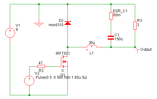
You can either load this circuit from EXAMPLES/SIMetrix/Tutorials/Tutorial2 (see Examples and Tutorials - Where are They?) or alternatively you can enter it from scratch. The latter approach is a useful exercise in using the schematic editor. To do this follow these instructions:
- Place the parts and wires as shown above.
- The probe labelled 'Output' can be selected from the following locations: The Part selector. If this is not already showing, select menu . Navigate to Probes ???MATH???\rightarrow???MATH??? Voltage Probe OR Menu OR Menu OR by pressing 'B' in the schematic editor.
- After placing the output probe, double click to edit its label. Enter Output in the box titled Curve Label. All the other options may be left at their defaults.
- For the pulse source V2, you can use or the Universal Source tool bar button.
-
Double click V2. Edit the settings as shown below:
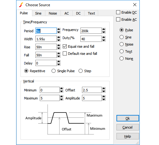 This sets up a 200kHz 5V pulse source with 40% duty cycle and 50nS rise time.
- Set up the simulation by selecting the schematic menu . In the dialog box, check Transient. Usually we would set the Stop time but on this occasion, the default 1mS is actually what we want. Now select the Advanced Options button. In the Integration method box, select Gear integration. This improves the simulation results for this type of circuit. You will still get sensible results without checking this option, they will just be a little better with it. (For more information, see Simulator Reference Manual/Convergence, Accuracy and Performance.
 The circuit is the switching stage of a simple step-down (buck) regulator designed to provide a 3.3 V supply from a 9V battery. The circuit has been stripped of everything except bare essentials in order to investigate power dissipation and current flow. Currently, it is a little over simplified as the inductor is ideal. More of this later. We will now make a few measurements. First, the power dissipation in Q1:
- Create an empty graph sheet by pressing F10
- Select schematic menu . Left click on Q1.
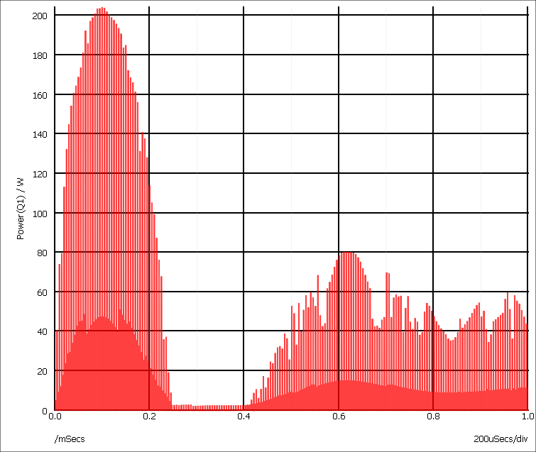
This shows a peak power dissipation of 200W although you are probably more interested in the average power dissipation over a specified time. To display the average power dissipation over the analysis period:
- Select menu
- Zoom in the graph at a point around 100uS, i.e. where the power dissipation is at a peak.
- Switch on graph cursors with menu . There are two cursors represented by cross-hairs. One uses a long dash and is referred to as the reference cursor, the other a shorter dash and is referred to as the main or measurement cursor. When first switched on the reference cursor is positioned to the left of the graph and the main to the right.
- Position the cursors to span a complete switching cycle. There are various ways of moving the cursors. To start with the simplest is to drag the vertical hairline left to right. As you bring the mouse cursor close to the vertical line you will notice the cursor shape change. See Graph Cursors for other ways of moving cursors.
-
Press F3 or select analysis menu :
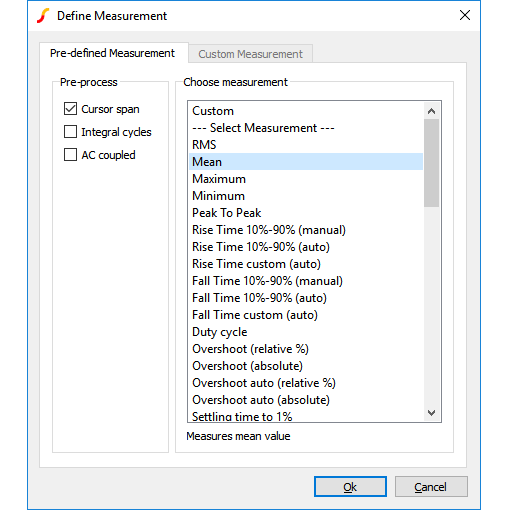
You should see a value of about 2.8W displayed. This is somewhat more than the 517mW average but is still well within the safe operating area of the device. However, as we noted earlier, the inductor is ideal and does not saturate. Lets have a look at the inductor current.
- Select schematic menu ...
- Left click on the left pin of the inductor L1. This is what you will see:
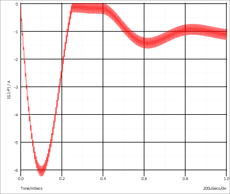 This shows that the operating current is less than 1.5A but peaks at over 6A. In practice you would want to use an inductor with a maximum current of around 2A in this application; an inductor with a 6A rating would not be cost-effective. We will now replace the ideal part, with something closer to a real inductor.
- Delete L1.
-
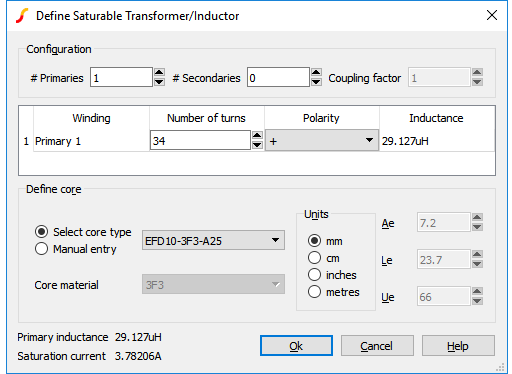
Select schematic menu . A dialog box will be displayed. (See picture below). Select 0 secondaries then enter 34 for the number of turns in primary 1. Next check Select Core Type. Select EFD10-3F3-A25. This is part number for a Ferroxcube ferrite core. This is what you should have:
 Click Ok to close the dialog box.
- Place the inductor in the same place as before.
- Run a new simulation.
- Select the graph sheet that displayed the inductor current by clicking on its tab at the top of the graph window. Now select schematic menu and left click on the left hand inductor pin.
- Select the graph sheet with the power plot then select ...
-
Zoom back to see the full graph using the zoom button.

- Zoom in on the peak power.
- Position the cursors to span a full cycle. (The cursors are currently tracking the first power curve. This doesn't actually matter here as we are only interested in the x-axis values. If you want to make the cursors track the green curve, you can simply pick up the cursor at its intersection with the mouse and drag it to the other curve).
-
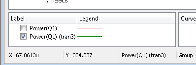
We now have two curves on the graph so we must select which one with which we wish to make the measurement. You can simply click on the curve to select it or check the box as shown below:
- As before, press F3 then select Mean with the cursor span pre-process option. The new peak power cycle will now be in the 11-12W region - much more than before.
| ◄ Tutorial 1 - A Simple Ready to Run Circuit | Tutorial 3 - Installing Third Party Models ▶ |