Optimizing the Deadtime for a Synchronous Buck Converter
In the previous section, Generating Efficiency Plots with Multi-Step Runs in DVM, you learned how to measure and plot the efficiency of the LLC converter over the line and load range. This is a classic verification example where the converter has already been designed and the testplan verifies the "goodness" of the design.
In this topic you will learn how to use DVM during the design process, that is, to optimize a particular design parameter using DVM. This kind of simulation is more akin to a Design of Experiments than a final verification. In this design of experiments, you will see how DVM can be used to analyze the deadtime for a synchronous buck converter.
To download the examples for the Applications Module, click Applications_Examples.zip
In this topic:
Key Concepts
- Testplans are easily modified and can be repurposed for other converters and tests.
- Even though the electrical ratings of two converters might be very different, testing the converters is similar.
- Using parameterization is critically important for design of experiments. Without a parameterized model, there is no way to vary critical design parameters.
What You Will Learn
In this topic, you will learn the following:
- How to modify an existing testplan.
Getting Started
To get started, open the schematic apps_d_2_buck_converter.sxsch. This schematic has been prepared to run DVM as described in the DVM Principles topic. The compensator design was taken directly from the SIMPLIS Tutorial, and a complete parameterized driver model has been added.
Exercise #1: Modify the Efficiency Testplan
The LLC converter used in the last example has an input voltage of 380V, and an output voltage of 24 volts at 120W. The synchronous buck converter design you just opened has a 12V input and 1.2V output at 12W. In this exercise you will see how easy it is to modify the LLC efficiency testplan to run on the synchronous buck converter. When modifying an existing testplan for a new schematic there are three areas to look out for:
- Hard-coded reference designators
- Hard-coded voltage, current, or other specification values.
- Pre and Post process scripts which might have hard-coded values.
Rename the Tesplan
- Open a Windows Explorer window in the Applications_Examples directory where you downloaded the schematic example files.
- Make a copy of the apps_d_1_llc_converter_efficiency.testplan file.
- Rename the copy to syncbuck_efficiency.testplan.
- Open the syncbuck_efficiency.testplan testplan in Excel.
Next, you will modify the testplan in Excel.
To get started, open the syncbuck_efficiency.testplan in a spreadsheet program. For reference, the testplan is shown below:
| *** | ||||||||
| *** apps_d_1_efficiency_multi_step.testplan | ||||||||
| *** | ||||||||
| *?@ Label | Objective | Analysis | Analysis | Change( V1.DC_VOLTAGE , 380 ) | Change( I1.LOAD_RESISTANCE , 5 ) | Create | Create | Postprocess |
| *** | ||||||||
| Efficiency|Step VIN and ILOAD | Steady-State | Multi-Step( ILOAD , LIN , 10 , 0.5 , 5.0 ) | Multi-Step( VIN , LIST , 360 , 380 , 400 ) | {VIN} | {RLOAD} | Alias( Efficiency , Efficiency_WHEN_VIN_%VIN% ) | Alias( Efficiency , Efficiency_WHEN_ILOAD_%ILOAD% ) | |
| Efficiency|Generate Efficiency Curves | NoSimulation | ./scripts/apps_d_1_create_xy_plots.sxscr | ||||||
Notice there are hard-coded reference designators V1 and I1 as well as hard-coded input voltage and output load current values in the Analysis columns. The hard-coded reference designators are not an issue in this case - the two schematics happen to have the same reference designators for the source and load. Also the postprocess script has the input voltage values hard-coded in it. In this example you will modify each value in turn.
- To start with, edit the Change() entries in cells E4 and F4 to use the parameterized {VIN} and {RLOAD} values respectively.
- Modify cell C6 to step the load current over 0.5A to 9.5A using the
Multi-Step( ILOAD , LIN , 10 , 0.5 , 9.5 , num_cores=4 )
entry.Note: This entry also uses a optional parameter string to set the number of cores to 4. If your machine has fewer than 4 cores, or your license doesn't support multi-core, the maximum number of cores will be used.
- Modify cell D6 to step the input voltage over a the list of 10.8, 12.0, and 13.2V with the Multi-Step( VIN , LIST , 10.8 , 12 , 13.2 ) entry.
- Change the name of the postproces script in cell I7 to ./scripts/apps_d_2_create_xy_plots.sxscr. This script is pre-prepared for the input voltages used in this converter.
- Delete the entire H column, this has the second alias for ILOAD : Alias( Efficiency , Efficiency_WHEN_ILOAD_%ILOAD% )
- Change the name of the testplan in cell A2 to *** syncbuck_efficiency.testplan.
- Save the file in tab-separated text format.
Your final testplan should look like the following, with changed elements in red text:
| *** | ||||||||
| *** syncbuck_efficiency.testplan | ||||||||
| *** | ||||||||
| *?@ Label | Objective | Analysis | Analysis | Change( V1.DC_VOLTAGE , {VIN} ) | Change( I1.LOAD_RESISTANCE , {RLOAD} ) | Create | Postprocess | |
| *** | ||||||||
| Efficiency|Step VIN and ILOAD | Steady-State | Multi-Step( ILOAD , LIN , 10 , 0.5 , 9.5 , num_cores=4 ) | Multi-Step( VIN , LIST , 10.8 , 12 , 13.2 ) | {VIN} | {RLOAD} | Alias( Efficiency , Efficiency_WHEN_VIN_%VIN% ) | ||
| Efficiency|Generate Efficiency Curves | NoSimulation | ./scripts/apps_d_2_create_xy_plots.sxscr | ||||||
Exercise #2: Run the Modified Testplan
Now you are ready to run this testplan on the schematic. To run the testplan,
- Select the .Result: A testplan file selection dialog opens.
- Navigate to the testplans directory
- Choose the syncbuck_efficiency.testplanResult: The entire testplan is run without prompting with a test selection dialog.
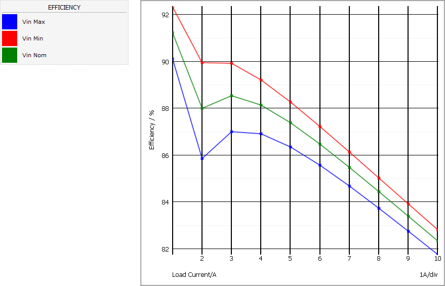
After the testplan executes you should see the efficiency curves for the converter, similar to:
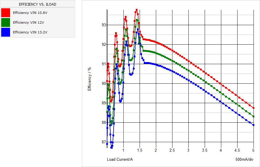
Before moving onto modifying the testplan to step the deadtime, a comment should be made on the number of data points used in these simulations. In the training course environment, users will have laptops with all sorts of processors and limitations - some computers will be very fast, others slow. For the purposes of demonstration during the class, we have chosen examples which simulate quickly. You should easily be able to modify these testplans to produce higher fidelity images, such as this one in which the ILOAD parameter was stepped from 0.5A to 5A in a decade sweep using 100 points per decade. The almost resonant effect seen in the low current efficiency is due to the discontinuous nature of the converter at light loads.
Exercise #3: Modify the Testplan to Step the Deadtime
Now that you have successfully modified the testplan to generate the efficiency curves for this converter, you will make a few more changes to the testplan to:
- Step the deadtime parameter DEADTIME_HSON.
- Set the input voltage to the nominal value.
- Call a slightly modified post process script to summarize the efficiency results. The postprocess script will generate a new curve for each deadtime with the efficiency on the vertical axis and the load current on the horizontal axis.
You can start with the testplan which you completed in the last section; however, it might be better to start with the pre-prepared apps_d_2_efficiency_multi_step.testplan file. This file should be identical to the one you modified and saved as syncbuck_efficiency.testplan. To avoid the complications of Excel mangling the filename, you will start by making a copy of the apps_d_2_efficiency_multi_step.testplan file in Windows Explorer. To get started, you will need to make a copy of the testplan
Rename the Testplan
- Open a Windows Explorer window in the Applications_Examples directory where you downloaded the schematic example files.
- Make a copy of the apps_d_2_efficiency_multi_step.testplan file.
- Rename the copy to syncbuck_efficiency_deadtime.testplan.
- Open the syncbuck_efficiency_deadtime.testplan testplan in Excel.
Next, you will modify the testplan in Excel.
Modify the Testplan
- To start with, edit the Change() entry in cell E4 from Change( V1.DC_VOLTAGE , {VIN} ) to Change( U2.DEADTIME_HSON , 10n ). This modification allows you to change the deadtime of the driver on a test by test basis.
- Insert an empty column before the Create entry in column G.
- Add a Source entry in cell G4.
- Modify the Label entry in cell A6, changing the label to Efficiency|Step DEADTIME_HSON and ILOAD.
- Modify the Multi-Step function in cell D6 to step the deadtime from 1ns to 8ns with the following Multi-Step function: Multi-Step( DEADTIME_HSON , LIN , 8 , 1n , 8n ).
- In the Change cell E6, enter {DEADTIME_HSON} to change parameterize the deadtime of the drivier.
- In the Source column, enter SOURCE( INPUT:1 , Nominal ). This tells DVM to change the value of the input source to the nominal value. The nominal voltage is read from the DVM control symbol.
- Change the Alias in cell H6 to Alias( Efficiency , Efficiency_WHEN_DEADTIME_HSON_%DEADTIME_HSON% )
- Change the name of the postprocess script in cell I7 to ./scripts/apps_d_3_create_xy_plots_for_deadtime.sxscr. This script is pre-prepared to plot the efficiency curves vs. deadtime in this converter.
- Change the name of the testplan in cell A2 to *** syncbuck_efficiency_deadtime.testplan.
- Save your testplan as tab-separated text with the new name, syncbuck_efficiency_deadtime.testplan.
Exercise #4: Run the Modified Testplan
Now you are ready to run this testplan on the schematic. To run the testplan,
- Select the .Result: A testplan file selection dialog opens.
- Navigate to the testplans directory
- Choose the syncbuck_efficiency_deadtime.testplanResult: The entire testplan is run without prompting with a test selection dialog.
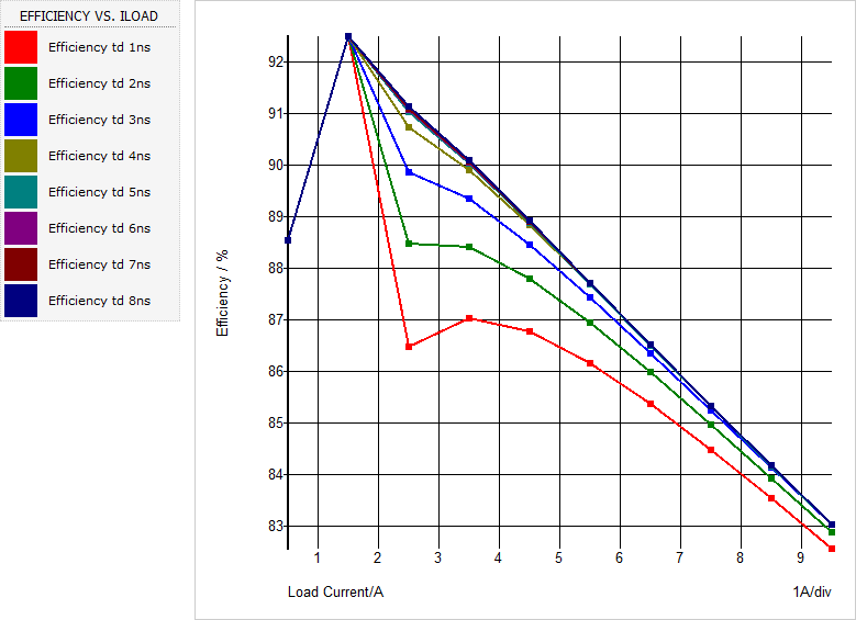
After the testplan executes you should see the efficiency curves for the converter, with the deadtime as the running parameter. Your curves should be similar to:
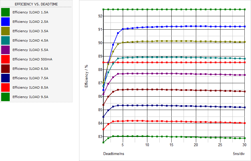
You can also "slice" the above data vertically by stepping the deadtime on the horizonal axis while the load current is the running parameter. In the graph below, the deadtime is stepped from 1ns to 30ns while the load current is stepped from 0.5 to 9.5A. The apps_d_4_efficiency_multi_step_step_deadtime_v_iload.testplan testplan was used to generate these curves.
Conclusions and Key Points to Remember
- Testplans are easily modified to change the goal of the simulation.
- Changing the stepped parameter name and values is quite easy, yet changes the goal of the simulation entirely.
- The number of cores can be defined in the testplan using an optional parameter string.