Cosine Waveform Load
The Cosine Waveform Load subcircuit models a time-varying load with a cosinusoidal current. At time=0, the load begins at the FINAL_CURRENT value and has a cosine function. The Cosine Waveform Load is not used in any test objectives, but you can change any load to a cosine load with a Cos() function call in a Load column.
Other similar loads include:
- Sine Load - similar to the Cosine Waveform Load but with a sine function.
In this topic:
| Model Name | Cosine Waveform Load | ||||
| Simulator |
|
This device is compatible with both the SIMetrix and SIMPLIS simulators. | |||
| Parts Selector Menu Location |
|
||||
| Symbol Library | None - the symbol is automatically generated when placed or edited. | ||||
| Model File | SIMPLIS_DVM_ADVANCED.lb | ||||
| Subcircuit Name |
|
||||
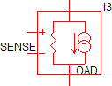
| Symbols |
|
||||
| Schematic - 2 Terminal |
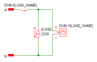
|
||||
| Schematic - 3 Terminal |
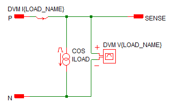
|
||||
| Schematic - 4 Terminal |
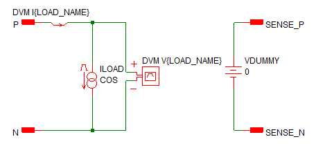
|
||||


Parameters
The following table explains the relevant parameters.
| Parameter Name | Default | Data Type | Range | Units | Parameter Description |
| COEFFICIENT | 0 | Real | The damping coefficient for the cosinusoidal load current. If non-zero, the cosinusoidal load current amplitude will decay with a time constant equal to ???MATH???\frac{1}{\text{COEFFICIENT}}???MATH???. | ||
| FINAL_CURRENT | 750m | Real | A | The peak or maximum current for the load. This can be a numeric value or a symbolic value, such as a percentage of full load. | |
| FREQUENCY | 10k | Real | min: > 0 | Hz | The frequency of the cosine waveform load |
| IDLE_IN_POP | 0 | Real | 0 or 1 | If set to 0, the load current during the POP analysis is set to the FINAL_CURRENT; otherwise, the load will be active during the POP analysis. | |
| LOAD_NAME | LOAD | String | n/a | n/a | Name of the DVM load. This name cannot contain spaces. |
| OFF_UNTIL_DELAY | 0 | Real | 0 or 1 | If set to 1, the load current will be ???MATH???\frac{1}{2}\left(\text{START_CURRENT}+\text{FINAL_CURRENT}\right)???MATH??? until the time specified by TIME_DELAY. If set to 0, the value of TIME_DELAY is interpreted as a phase delay. | |
| PHASE_ANGLE | 90 | Real | ° | The phase angle of the cosinusoidal waveform, used only if the USE_PHASE parameter is 1. | |
| START_CURRENT | 0 | Real | A | The minimum or starting current for the cosine waveform load. This can be a numeric value or a symbolic value, such as a percentage of full load. | |
| TIME_DELAY | 10u | Real | min: 0 | s | The delay before the cosinusoid starts. The load behavior before the TIME_DELAY is determined by the OFF_UNTIL_DELAY parameter. |
| USE_PHASE | 0 | Real | 0 or 1 | If set to 1, the load is configured to use the phase angle supplied by the PHASE_ANGLE parameter. |
Testplan Entry
To set any managed DVM load to a Cosine Waveform Load subcircuit, place a Cos() testplan entry in a Load column.
The Cos() testplan entry has the following syntax with the arguments taken from the list of parameters above.
Cos(REF, START_CURRENT, FINAL_CURRENT, FREQUENCY)
Cos(REF, START_CURRENT, FINAL_CURRENT, FREQUENCY, OPTIONAL_PARAMETER_STRING)
| Argument | Range | Description |
| REF | n/a | The actual reference designator of the DVM load or the more generic syntax of OUTPUT:n where n is an integer indicating a position in the list of managed DVM loads. |
| START_CURRENT | n/a | The minimum or starting current for the cosine waveform load. This can be a numeric value or a symbolic value, such as a percentage of full load. |
| FINAL_CURRENT | n/a | The peak or maximum current for the cosine wave load. This can be a numeric value or a symbolic value, such as a percentage of full load. |
| FREQUENCY | min: > 0 | The frequency of the cosine waveform load. |
| OPTIONAL_PARAMETER_STRING | n/a | Parameter string with any of the other parameters from the parameter table above* |
* If multiple parameters are specified, join the parameter key-value pairs with a space, as shown in the examples below. The order of the parameter names does not matter.
Examples
The following three examples set the first DVM managed load to a Cosine Waveform Load with a minimum current of 0A and a peak current of 1A. The timing parameters and the optional parameter strings are different in each example.
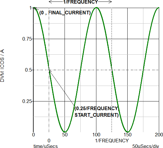
Zero Time Delay Example
Since the TIME_DELAY parameter is set to zero in this example, the cosine wave begins with the FINAL_CURRENT value of 1A at t=0.
| *?@ Load |
|---|
| Cos(OUTPUT:1, 0, 1, 10k, TIME_DELAY=0) |
The results of this testplan entry are shown below:
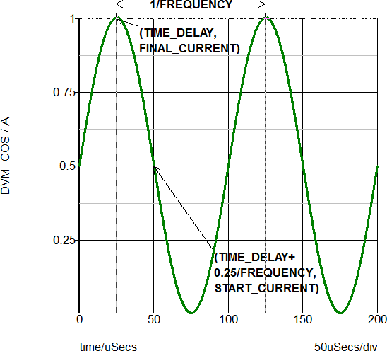
Time Delay Example
In this example, the TIME_DELAY parameter is set to 25us. Since the OFF_UNTIL_DELAY parameter is not specified, the TIME_DELAY value is interpreted as a phase delay. This results in the same waveform as a Sine Waveform Load.
| *?@ Load |
|---|
| Cos(OUTPUT:1, 0, 1, 10k, TIME_DELAY=25u) |
The results of this testplan entry are shown below:
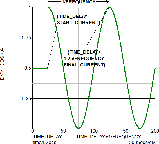
Time Delay Example With OFF_UNTIL_DELAY=1
In this example, the TIME_DELAY parameter is set to 25us, and the OFF_UNTIL_DELAY is set to 1; therefore, for simulation times less than the TIME_DELAY parameter, the load current is 0.5A, as determined by the following equation: ???MATH???\frac{1}{2}\left(\text{START_CURRENT}+\text{FINAL_CURRENT}\right)???MATH???
| *?@ Load |
|---|
| Cos(OUTPUT:1, 0, 1, 10k, TIME_DELAY=25u OFF_UNTIL_DELAY=1) |
The results of this testplan entry are shown below: