Accuracy and Integration Methods
In this topic:
A Simple Approach
If you wish to increase the accuracy of a simulation, reduce the value of RELTOL. This defaults to 0.001 so to reduce it to say 1e-5 add the following line to the netlist:
.OPTIONS RELTOL=1e-5
(The setting of RELTOL is supported by the front end. See User's Manual/Analysis Modes/Simulator Options/Setting Simulator Options/Tolerances for details.)
The simulation will run slower. It might be a lot slower it might be only slightly slower. In very unfortunate circumstances it might not simulate at all and fail with a convergence error.
Conversely, you can speed up the simulation by increasing RELTOL but you should not set this to a value higher than around 0.005 as this will degrade accuracy to an unacceptable level.
Iteration Accuracy
For DC and transient modes, the simulator essentially makes an approximation to the true answer. For DC analysis an iterative method is used to solve the non-linear equations which can only find the exact answer if the circuit is linear. The accuracy of the result for non-linear circuits is determined by the number of iterations; accuracy is improved by performing more iterations but obviously this takes longer. In order to control the number of iterations that are performed an estimate is made of the error by comparing two successive iterations. When this error falls below a predetermined tolerance, the iteration is deemed to have converged and the simulator moves on the next step or completes the run. Most SPICE simulators use something similar to the following equations to calculate the tolerance:
For voltages: TOL = RELTOL * instantaneous_value + VNTOL
For currents: TOL = RELTOL * instantaneous_value + ABSTOL
"instantaneous_value" is the larger of the current and previous iterations. VNTOL has a default value of 1???MATH???\mu???MATH???V so for voltages above 1mV, RELTOL dominates. ABSTOL has a default of 1pA so for currents above 1nA, RELTOL dominates.
The above method of calculating tolerance works fine for many circuits using the default values of VNTOL and ABSTOL. However, SPICE was originally designed for integrated circuit design where voltages and currents are always small, so the default values of ABSTOL and VNTOL may not be appropriate for - say - a 100V 20A power supply. Suppose, that such a PSU has a current that rises to 20A at some point in the simulation, but falls away to zero. When at 20A it has a tolerance of 20mA but when it falls to zero the tolerance drops to ABSTOL which is 1pA. In most situations the 1pA tolerance would be absurdly tight and would slow down the simulation. Most other SPICE products recommend increasing ABSTOL and VNTOL for PSU circuits and indeed this is perfectly sound advice. However, In SIMetrix the tolerance equation has been modified to make this unnecessary in most cases. Here is the modified equation:
For voltages: TOL = RELTOL * MAX( peak_value * POINTTOL, instantaneous_value ) + VNTOL
For currents: TOL = RELTOL * MAX( peak_value * POINTTOL, instantaneous_value ) + ABSTOL
peak_value is the magnitude of the largest voltage or current encountered so far for the signal under test. POINTTOL is a new tolerance parameter and has a default value of 0.001. So for the example we gave above, peak_value would be 20 and when instantaneous_value falls to zero the tolerance would be:
0.001 * MAX(20 * 0.001, 0) + 1p = approx. 20???MATH???\mu???MATH???A
20???MATH???\mu???MATH???A is a much more reasonable tolerance for a signal that reaches 20A.
The above method has the advantage that it loosens the tolerance only for signals that actually reach large values. Parts of a circuit that only see small voltages or currents - such as the error amplifier of a servo-controlled power supply - would still be simulated with appropriate precision.
POINTTOL can be increased to improve simulation speed. It is a more controlled method than increasing RELTOL. POINTTOL can be raised to 0.1 or even 1.0 but definitely no higher than 1.0.
Time Step Control
The tolerance options mentioned above also affect the time step control algorithm used in transient analysis. In SIMetrix, there are three mechanisms that control the time step, one of which has to be explicitly enabled. These are:
- Iteration time step control
- LTE time step control
- Voltage delta limit
Iteration Time Step Control
Iteration control reduces the time step by a factor of 8 if convergence to the specified accuracy cannot be achieved after 10 iterations. (10 by default but can be changed with ITL4 option). If convergence is successful, the time step is doubled. As this mechanism is controlled by the success or otherwise of the iteration it is also affected by the same tolerance options described in the above section about iteration accuracy.
LTE Time Step Control
"LTE time step control" is an algorithm which controls the accuracy of the numerical integration method used to model reactive devices such as inductors and capacitors. These devices are governed by a differential equation. It is not possible in a non-linear circuit to solve these differential equations exactly so a numerical method is used and this - like the iterative methods used for non-linear devices - is approximate. In the case of numerical integration, the accuracy is determined by the time step. The smaller the time step the greater the accuracy but also the longer the simulation time.
The accuracy to which capacitors are simulated is controlled by RELTOL, POINTTOL and two other options namely TRTOL and CHGTOL. The latter is a charge tolerance and has a similar effect to VNTOL and ABSTOL but instead represents the charge in the capacitor. It's default value is 1e-14 which, like ABSTOL and VNTOL is appropriate for integrated circuits but may be too low for PSU circuits with large capacitors. However, the peak detection mechanism controlled by POINTTOL described in the above section also works for the LTE time step control algorithm and it is therefore rarely necessary to alter CHGTOL.
TRTOL is a dimensionless value which defaults to 7. It affects the overall accuracy of the numerical integration without affecting the precision of the iteration. So reducing TRTOL will increase the accuracy with which capacitors and inductors are simulated without affecting the accuracy of the iterative method used to simulate non-linear elements. However, in order for the simulation of reactive devices to be accurate, the non-linear iteration must also be accurate. So, reducing TRTOL much below unity will result in a longer simulation time but no improvement in precision. Increasing TRTOL to a large value, however, may be appropriate in some circumstances where the accuracy to which reactive devices are simulated is not that important. This may be the case in a circuit where there is an interest in the steady state but not in how it was reached.
Inductors are controlled by the same tolerances except CHGTOL is replaced by FLUXTOL. This defaults to 1e-11.
The default LTE time step algorithm used in SIMetrix is slightly different to that used by standard SPICE. The standard SPICE variant is also affected by ABSTOL and VNTOL. The SIMetrix algorithm controls the time step more accurately and as a result offers better speed-accuracy performance.
Voltage Delta Limit
This places a limit on the amount of change allowed in a single timestep for each node. This limit is governed by the option setting MAXVDELTAREL and MAXVDELTAABS and is included to overcome a problem that can cause false clocking of flip-flops. The limit can be calculated from:
MAXVDELTAABS + MAXVDELTAREL*(node_voltage)
where node_voltage is the larger of the node voltage at current time step and the node voltage at the previous time step. The above is calculated for all voltage nodes. If the change in voltage exceeds this limit, the time step is cut back.
The above mechanism is not enabled if MAXVDELTAREL is zero or less and MAXVDELTAREL is zero by default.
Setting MAXVDELTAREL to a value of about 0.4 will usually fix problems of false clocking in flip-flops. However, this will slow down the simulation slightly and it is not recommended that this setting is used in circuits that do not contain flip-flops.
Accuracy of AC analyses
The small-signal analysis modes .AC, .TF and .NOISE do not use approximate methods and their accuracy is limited only by the precision of the processor's floating point unit. Of course the DC operating point that always precedes these analysis modes is subject to the limitations described above. Also, the device models used for non-linear devices are also in themselves approximations. So these modes should not be seen as exact but they are not affected by any of the tolerance option settings.
Summary of Tolerance Options
RELTOL
Default = 0.001. This affects all DC and transient simulation modes and specifies the relative accuracy. Reduce this value to improve precision at the expense of simulation speed. We do not recommend increasing this value except perhaps to run a quick test. In any case, you should never use a value larger than 0.01.
POINTTOL
Proprietary to SIMetrix. Default = 0.001. Can increase to a maximum of 1.0 to improve speed with loss of precision. Reduce to 0 for maximum accuracy but note this may just slow down the simulation without really improving precision where it is needed.
ABSTOL
Default = 1pA. This is an absolute tolerance for currents and therefore has units of Amps. This basically affects the tolerance for very low values of current. Sometimes worth increasing to resolve convergence problems or improve speed for power circuits.
VNTOL
Default = 1V. Same as ABSTOL but for voltages.
TRTOL
Default = 7. This is a relative value and affects how accurately charge storage elements are simulated. Reduce it to increase accuracy of reactive elements but there is no benefit reducing below about 1.0. In circuits where there is more interest in the steady state rather than how to get there, simulation speed can be improved by increasing this value.
CHGTOL
Default = 1e-14. Minimum tolerance of capacitor charge. Some convergence and speed improvement may be gained by increasing this for circuits with large capacitors. Generally recommended to leave it alone.
FLUXTOL
Default = 1e-11. Same as CHGTOL except applied to inductors.
Integration Methods - METHOD option
SIMetrix, along with most other SPICE products use three different numerical integration methods to model reactive elements such as capacitors and inductors. These are Backward Euler, Trapezoidal Rule and Gear. Backward Euler is used unconditionally at various times during the course of a simulation but at all other times the method used is controlled by the METHOD option (as long as ORDER is set to 2 or higher - see below).
The METHOD option can be set to TRAP (trapezoidal - the default) or GEAR. Gear integration can solve a common problem whereby the solution seems to oscillate slightly. An example is shown below.
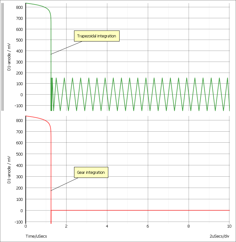
The plots show the reverse recovery of a diode. The green curve was simulated with the default trapezoidal integration method whereas the red used Gear integration. Note that gear integration introduces a slight overshoot. This is a common characteristic. To find out whether such overshoots are a consequence of the integration or are in fact a real circuit characteristic, you should simulate the circuit with much smaller values of RELTOL (see above). It is also suggested that you switch back to trapezoid integration when using tight tolerances; the oscillation caused by trapezoidal integration disappear if the time step falls below half the time constant of the circuit.
Note, you should not use Gear integration if you are simulating strongly resonant circuits such as oscillators. Gear integration introduces a numerical damping effect which will cause resonant circuits to decay more rapidly than they should. For example:
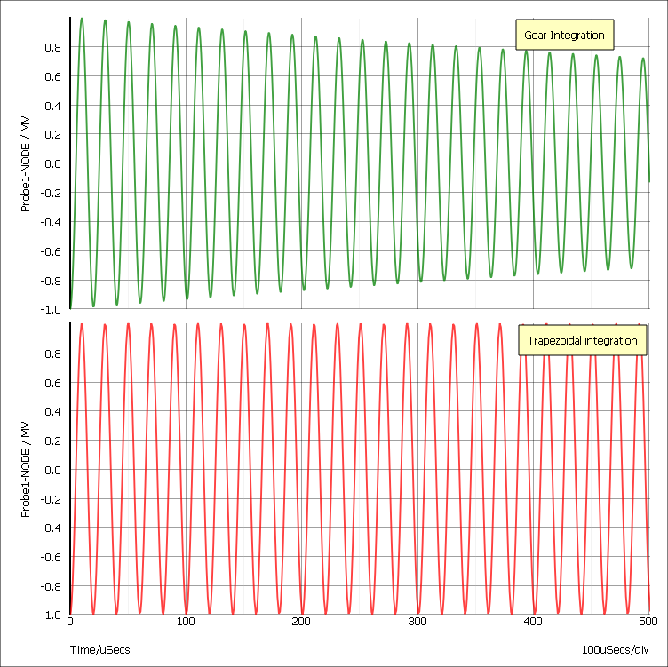
The above curves are the result of simulating a simple LC circuit that is completely undamped. The top trace was the result of Gear integration and the bottom, trapezoidal. The bottom curve is correct and agrees with theory. The top curve is inaccurate. If the analysis was done with Gear integration but with a smaller value of RELTOL, the damping effect would be less, so for all methods the result is ultimately accurate if the tolerance is made small enough. But trapezoidal gives accurate results without tight values of RELTOL.
ORDER option
This defaults to 2 and in general we recommend that it stays that way. Setting it to 1 will force Backward Euler to be used throughout which will degrade precision without any speed improvement. It can be increased up to a value of 6 if METHOD=GEAR but we have not found any circuits where this offers any improvement in either speed or precision.
| ◄ Transient Analysis - 'Time step too small' Error | Using Multiple Core Systems ▶ |