Transient Analysis
In this mode the simulator computes the behaviour of the circuit over a time interval specified by the stop time. Usually, the stop time is the only parameter that needs specifying but there are a number of others available.
In this topic:
Setting up a Transient Analysis
- Select menu
- Select Transient check box on the right.
- Select Transient tab at the top. Enter parameters as described in the following sections.
Transient Parameters
Enter the stop time as required. Note that the simulation can be paused before the stop time is reached allowing the results obtained so far to be examined. It is also possible to restart the simulation after the stop time has been reached and continue for as long as is needed. For these reasons, it is not so important to get the stop time absolutely right. You should be aware, however, that the default values for a number of simulator parameters are chosen according to the stop time. (The minimum time step for example). You should avoid therefore entering inappropriate values for stop time.
Data Output Options
Sometimes it is desirable to restrict the amount of data being generated by the simulator which in some situations can be very large. You can specify that data output does not begin until after some specified time and you can also specify a time interval for the data.
Output all data/Output at .PRINT step
The simulator generates data at a variable time step according to circuit activity. If Output all data is checked, all this data is output. If Output at .PRINT step is checked, the data is output at a fixed time step regardless of the activity in the circuit. The actual interval is set by the .PRINT step. This is explained below.
If the Output at .PRINT step option is checked, the simulator is forced to perform an additional step at the required interval for the data output. The fixed time step interval data is not generated by interpolation as is the case with generic SPICE and other products derived from it.
Start data output @
No simulation data will be output until this time is reached.
.PRINT step
.PRINT is a simulator command that can be specified in the netlist to enable the output of tabulated data in the list file. See Simulator Reference Manual/Command Reference/.PRINT for details of .PRINT.
The value specified here controls the interval used for the tabulated output provided by .PRINT but the same value is also used to determine the data output interval if Output at .PRINT step is specified.
Real Time Noise
See Real Time Noise.
Monte Carlo and Multi-step Analysis
Advanced Options
Opens a dialog as shown below
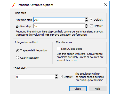
Time Step
The options presented here set upper and lower limits to the time step used in transient analyis. It is important to note that the behaviour of the lower limit is different to the upper limit. The actual time step used is controlled by the simulator to ensure convergence and to satisfy tolerance requirements. It will not set a limit higher than the upper limit, but if it needs to set a time step below the lower limit, the simulation will abort; it will not simply hold the time step at the lower limit.
Time step too smallerror.
Integration Method
Set this to Gear if you see an unexplained triangular ringing in the simulation results. Always use Trapezoidal for resonant circuits. A full discussion on integration methods is given in the Simulator Reference Manual:Convergence, Accuracy and Performance/Accuracy and Integration Methods/Integration Methods - METHOD option.
Skip DC bias point
If checked, the simulation will start with all nodes at zero volts. Note that unless all voltage and current sources are specified to have zero output at time zero, the simulation may fail to converge if this option is specified.
Fast start
The accuracy of the simulation will be relaxed for the period specified. This will speed up the run at the expense of precision.
This is a means of accelerating the process of finding a steady state in circuits such as oscillators and switching power supplies. Its often of little interest how the steady state is reached so precision can be relaxed while finding it.
Note that the reduced precision can also reduce the accuracy at which a steady state is found and often a settling time is required after the fast start period.
Restarting a Transient Run
After a transient analysis has run to completion, that is it has reached its stop time, it is still possible to restart the analysis to carry on from where it previously stopped. To restart a transient run:
- Select the menu .
- In the New Stop Time box enter the time at which you wish the restarted analysis to stop. Click Ok to start run.
See Also
Transient Snapshots
Overview
There is often a need to investigate a circuit at a set of circuit conditions that can only be achieved during a transient run.
For example, you might find that an amplifier circuit oscillates under some conditions but these conditions are difficult or impossible to create during the bias point calculation that usually precedes a small-signal AC analysis.
Transient snapshots provide a solution to this problem. The state of the circuit at user specified points during a transient run may be saved and subsequently used to initialise a small-signal analysis. The saved state of the circuit is called a snapshot.
Snapshots can be created at specified intervals during a transient run. They can also be created on demand at any point during a transient run by first pausing the run and then manually executing the save snapshot command. So, for example, if you find your amplifier reaches an unstable point during a transient analysis, you can stop the analysis, save a snapshot and then subsequently analyse the small signal conditions with an AC sweep.
An option is also available to save the DC operating point data to the list file at the point at which snapshots are saved.
Defining Snapshots Before a Run Starts
- Select menu
- In the Transient Sheet select button Define Snapshots...
- You will see the following dialog
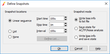 Select either Linear sequence
or List
to define the time points at which the snapshots are saved. In the Snapshot mode box select one of the three options:
Select either Linear sequence
or List
to define the time points at which the snapshots are saved. In the Snapshot mode box select one of the three options:
- Write bias info to list file. Instructs the simulator to write the DC operating point data to the list file. Does not save snapshot data.
- Save state for AC/TF/Noise analysis. Instructs the simulator to save snapshot data only. No bias point information will be output to the list file.
- Write bias info and save state. Performs both operations described in 1 and 2 above.
Creating Snapshots on Demand
You can create a snapshot of a transient run after it has started by executing the SaveSnapShot script command. Proceed as follows:
- Pause the current transient analysis or allow it to finish normally. You must not abort the run as this destroys all internal simulation data.
-
Type at the command line (the edit box at the top of the command shell):
SaveSnapShot
Applying Snapshots to a Small Signal Analysis
- Select menu
- Select AC, TF or Noise analysis
- Press Define Multi-step Analysis for the required analysis mode.
- Select Snapshot mode.
Important Note
Snapshot data can only be applied to an identical circuit to the one that created the snapshot data. So, you must make sure that any parts needed for a small-signal analysis that uses snapshot data are already present in the circuit before the transient run starts. In particular, of course, you must make sure that an AC source is present.
An error message will be output if there are any topological differences between the circuit that generated the snapshot data and the circuit that uses it. If there are only part value or model parameter differences, then the snapshot data may be accepted without error but at best the results will need careful interpretation and at worst will be completely erroneous. Generally, if you change a part that affects the DC operating point then the results will not be meaningful. If you change only an AC value, e.g. a capacitor value, then the results will probably be valid.
How Snapshots are Stored
The snapshot data is stored in a file which has the default name of netlist.sxsnp where netlist is the name of the netlist used for the simulation. When using the schematic editor, this is usually design.net so the usual name for the snapshot file is design.sxsnp. You can override this name using the SNAPSHOTFILE OPTIONS setting although there is rarely any reason to do this.
The snapshot file is automatically deleted at the start of every transient run. The SaveSnapShot command always appends its data to the snapshot file so that any pre-defined snapshots are preserved.
When snapshot data is applied to a subsequent small-signal analysis, the snapshot file is read and checked that it is valid for the circuit being analysed.
| ◄ Running Simulations | Operating Point ▶ |