Synopsis of Small-Signal AC Analysis
After the periodic-operating point/trajectory of the system has been determined by the periodic-operating point (POP) analysis, the SIMPLIS-FX Small-Signal Frequency-Domain Analysis can then be applied to compute the small-signal response of the system in a small neighborhood around the large-signal periodic equilibrium. For illustration purposes, let us assume that the following .AC analysis statement was specified in the input file:
.AC DEC 10 250 25K
This analysis statement instructs SIMPLIS-FX to carry out the small-signal frequency-domain analysis by sweeping the excitation frequency of all small-signal AC sources in a logarithmic manner from 250 Hz to 25 kHz. The number of analysis frequencies per decade is set to 10. You can easily verify that this analysis statement leads to the following excitation frequencies:
250.000 Hz 314.731 Hz 396.223 Hz
. . .
1.57739 kHz 1.98582 kHz 2.50000 kHz
3.14731 kHz 3.96223 kHz
. . .
15.7739 kHz 19.8582 kHz 25.0000 kHz
As the sequence of small-signal analyses at these excitation frequencies is carried out, SIMPLIS-FX reports the progress by printing a matrix of numbers which represent the "percent complete" of the swept-frequency analysis. For example, a screen display such as:
SMALL-SIGNAL FREQUENCY-DOMAIN ANALYSIS
CONTINUOUS S-DOMAIN

01 02 03 04 05 06 07 08 09 10
11 12 13 14 15 16 17 18 19 20
21 22 23 24 25 26 27 28 29 30
31 32 33 34 35 36 37 38 39 40
41 42 43 44 45 46 47 48 49 50
51 52
Elapsed time : 0 hr 0 min 6 sec
CPU time : 0 hr 0 min 4.64 sec
Analyzed freq. : 2.500000000000e+03 Hz
means that 52 percent of the small-signal frequency-domain analyses have been completed and that the excitation frequency has been swept past 2.5 kHz.
The "percent complete" shown in the small-signal frequency-domain analysis is calculated based on the number of expected analyses at discrete excitation frequencies and not based on the CPU time. Since a logarithm sweep of 10 points per decade from 250 Hz to 25 kHz is specified in the preceding example, there will be a total of 21 analyses starting from 250 Hz and stopping at 25 kHz. The analysis at 2.5 kHz is the 11th one in this sequence of analyses. Hence, if SIMPLIS-FX has just finished the analysis at 2.5 kHz, the percent complete is reported as (11 / 21) x 100 = 52%.
The actual CPU time involved in each individual analysis varies. As a rule of thumb, the CPU time is linearly proportional to the excitation frequency. When the excitation frequency is 1 decade or more below the periodic operating frequency computed in the POP analysis, SIMPLIS-FX is extremely fast. When the excitation frequency is close to the periodic operating frequency computed in the POP analysis, SIMPLIS-FX is reasonable in computation speed. When the excitation frequency is 1 decade or more above the periodic operating frequency computed in the POP analysis, the computation time taken by SIMPLIS-FX will be much longer, since SIMPLIS-FX must determine the high excitation frequency affect on the system response.
This brief synopsis is adequate as a reference for using the SIMPLIS-FX Small-Signal Frequency-Domain Analyzer. It is recommended that any first-time user, as well as those interested in more details of SIMPLIS-FX, read the following subsections of this Section to better understand the behavior of small-signal AC sources and various large-signal time-varying sources during the small-signal frequency-domain analysis. Behaviour of AC Sources in Transient and POP describes how the small-signal AC sources are treated in both the time-domain transient analysis and the periodic operating-point analysis.
In this topic:
Amplitude of Small-Signal AC Sources
If the continuous domain is chosen for the small-signal frequency-domain analysis, all of the small-signal AC sources are sinusoids. If the discrete domain is chosen instead, the waveforms of all of the small-signal AC sources are the result of applying a sample-and-hold process to a sinusoid. In both cases the original sinusoidal waveform is completely defined by three parameters: the frequency, the amplitude, and the phase of the sinusoidal waveform. The frequency of each small-signal AC source is set to the analysis frequency defined by the "sweep_type" and "n_pt" parameters in the .AC analysis statement. The "amplitude" parameter is explained in this subsection.
The "amplitude" parameter in the device statement defining a small-signal AC source should be regarded as a relative quantity rather than an absolute quantity. Suppose the following statements appear in the input file:
V1 1 0 AC 2 -45 V2 4 0 AC I3 7 9 AC 5 60
Since the amplitude and the phase parameters of V2 are not specified, the defaults of 1.0 unit and 0.0 degree are used. Although the amplitude parameter of V1 is set to 2, the actual amplitude of V1 during the small-signal frequency-domain analysis is not equal to 2.0 V. By definition, a small-signal analysis is the examination of the behavior of a system around its equilibrium when it is perturbed from its equilibrium with stimuli of infinitesimally small amplitude. The amplitude of the three sources V1, V2, and I3 are all set to infinitesimally small values by SIMPLIS-FX during the small-signal analysis. However, the ratios between the amplitude of these three sources are maintained according to the amplitude parameters in the statements defining the small-signal AC sources. In this example, the amplitude of V1 is always set to twice the amplitude of V2 and the amplitude of I3 is always set to five times as large as the amplitude of V2. Another way to interpret the three device statements above is that the amplitude of V1, V2, and I3 are 2, 1, and 5 infinitesimally small units, respectively.
The excitation of a nonlinear system by sinusoidal inputs with finite amplitudes generates responses not only at the excitation frequency, but also at harmonics or subharmonics of the excitation frequency. For a true small-signal analysis, the amplitude of the sinusoidal inputs must be made infinitesimally small so the responses at the higher harmonics and/or the subharmonics are insignificant compared to the response at the excitation frequency. This is equivalent to saying that the response of a nonlinear system appears linear when the amplitude of the excitation sources are sufficiently small. The same can be said about switching piecewise-linear systems.
Making small-signal measurements on a breadboard system in the laboratory presents some practical challenges in choosing the amplitude of the exciting sinusoids. Ideally, we would like the amplitude of the exciting sinusoids to be as small as possible to avoid the nonlinear effects, but the amplitude of these exciting sinusoids cannot be too small. If these amplitudes are too small, the signal-to-noise ratio would be low and it will be extremely difficult to get an accurate measurement. This is especially true for switching systems which inherently carry large-signal noises at the switching frequency and higher harmonics. SIMPLIS-FX uses a proprietary algorithm to make sure that the amplitude of all small-signal AC sources are infinitesimally small so as to generate linear responses, and the infinitesimally small responses are accurately resolved in the presence of the large-signal switching noises.
Phase Delay of Small-Signal AC Sources
Similar to the "amplitude" parameter, the "phase" parameter in the device statements defining a small-signal AC source is a relative quantity rather than an absolute quantity. Suppose again that the following device statements appear in the input file:
V1 1 0 AC 2 -45 V2 4 0 AC I3 7 9 AC 5 60
The amplitude and the phase parameters of V2 are not specified, so the default values of 1.0 unit and 0.0 degree are used. The phase parameter is a relative quantity. In this example, the phase of I3 is set to 60 degrees ahead of the phase of V2 at any excitation frequency, and the phase of V1 is set to 45 degrees behind the phase of V2.
You will rarely need more than one small-signal AC source with different phase delay in the small-signal frequency-domain analysis of switching piecewise-linear systems. The phase parameter has been provided for backward compatibility with existing circuit simulators such as SPICE.
Sample Waveforms of AC Sources Continuous Domain
The waveform of a small-signal AC source is sinusoidal if the continuous domain is used for the small-signal frequency-domain analysis. For example, the following device statements specify three small-signal AC sources V1, V2, and I3 with amplitudes equal to 2, 1, and 5 units, respectively.
V1 1 0 AC 2 -45 V2 4 0 AC I3 7 9 AC 5 60
The waveforms of these three sources at an analysis frequency of 1 kHz are displayed in 11.1(a). The waveforms of these sources at an analysis frequency of 2 kHz are displayed in 11.1(b). Since the phase parameter is relative, these waveforms have been arbitrarily drawn with V2 having a positive-slope zero crossing at t=0. Once the phase of V2 has been arbitrarily chosen, the phases of V1 and I3 are fixed at 45 degrees behind and 60 degrees ahead of the phase of V2, respectively.
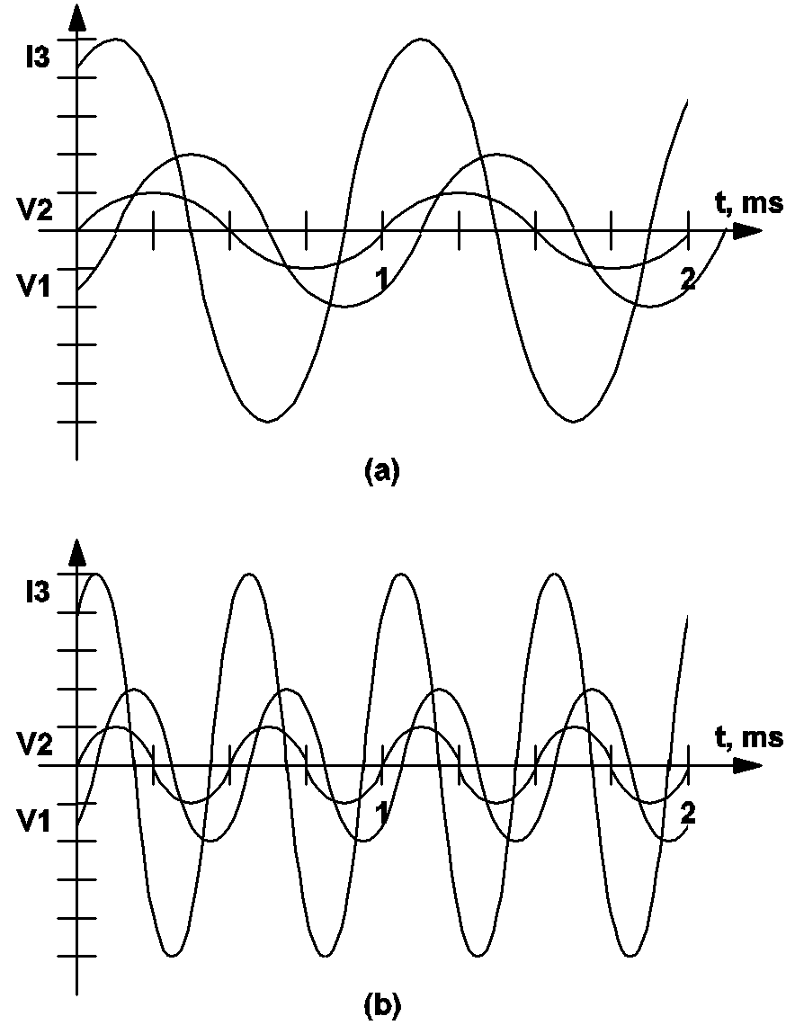 |
11.1 Waveforms for the small-signal AC source examples V1, V2, and I3. |
Sample Waveforms of AC Sources Discrete Domain
If the discrete domain is used, the waveform of a small-signal AC source as a function of time is the result of applying an ideal sample-and-hold process to a sinusoidal waveform. This ideal sampling is taken at the beginning of a switching period/cycle where the beginning of a switching period/cycle is defined through the .POP analysis statement. The value of a small-signal AC source is held constant for the remaining of the switching period/cycle until another set of samples is taken at the start of the next switching period/cycle. The sample device statements shown in Sample Waveforms of AC Sources Continuous Domain are repeated here for illustration:
V1 1 0 AC 2 -45 V2 4 0 AC I3 7 9 AC 5 60
Suppose the analysis frequency is 1 kHz and the switching frequency, or the periodic operating frequency, computed by the POP analysis is 50 kHz. Fig. 11-2(a) shows the sinusoidal waveforms associated with V1 and I3 in dash lines and their actual waveforms in solid lines. It can be seen that the waveforms of V1 and I3 are obtained by applying sample-and-hold to the corresponding sinusoidal waveforms. The associated waveforms of V2 are expressly omitted in fig 11.2 (a) to reduce the cluttering of the figure. The waveforms associated with V1 and I3 should sufficiently illustrate the sample-and-hold process. Fig 11.2(b) show similar waveforms of V1 and I3 when the analysis frequency is at 2 kHz.
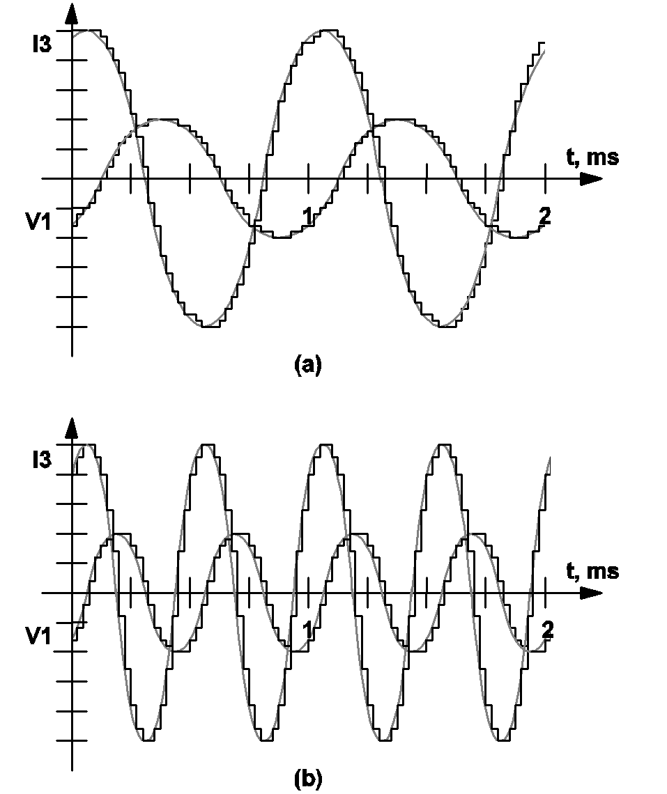 |
11.2 Waveforms for the small-signal AC source examples, V1 and I3. |
Continuous and Discrete Domain Differences
The most obvious difference between using the continuous domain or the discrete domain in the small-signal analysis is the source values of the small-signal AC sources. As illustrated in the previous subsections, the source value of a small-signal AC source is a continuous sinusoidal waveform if the continuous domain is used. If the discrete domain is used, the waveform of a small-signal AC source is the piecewise-constant waveform resulting from the application of a sample-and-hold to a related continuous sinusoidal waveform.
Another difference between using the continuous domain and the discrete domain in the small-signal analysis is the way the responses are analyzed. In the case of the continuous domain, Fourier analysis is directly applied to any response of the system to extract the harmonic with the same frequency as the analysis frequency. In the case of the discrete domain, a sample-and-hold process is applied to each response of the system, and Fourier analysis is then applied to the result of this sample-and-hold process. The sampling is set to occur, just like the small-signal AC sources, at the beginning of a switching cycle where this beginning is defined through the .POP analysis statement.
Whether continuous domain or discrete domain is used, the effects of the implicit sample-and-hold that occurs in a switching system are taken into consideration by SIMPLIS-FX. For example, if a simple switch, S, is controlled by a control signal, cs(t), an effective sample-and-hold process of cs(t) is taken place at every moment switch S switches position.
Another example of implicit sample-and-hold occurs at the two inputs of a comparator. Whenever the comparator switches its output logic state, we have, in effect, a sample-and-hold of the two analog inputs of the comparator. If you are familiar with the peak-current control of energy-storage dc-to-dc converters, recall that peak-current control would approach unstable operation as the duty ratio of the power switch approaches 50%, provided no compensation ramp is applied to the control. Using existing modeling methods, such instability can only be predicted by explicitly adding a sample-and-hold function block, or any approximation of such, from the controlling signal to the power stage. Such explicit addition is not necessary when these control strategies are analyzed with SIMPLIS-FX because the implicit sample-and-hold process that occurs in the circuit is taken into consideration in the computation of the frequency response. As a result, the schematic that is used for time-domain simulation is the schematic that will be analyzed in frequency-domain, eliminating the need to replace parts of a schematic by averaged-circuit equivalents and eliminating the need to add extraneous components or function blocks when small-signal frequency-domain analysis is performed. Using SIMPLIS-FX, you can study how a converter under peak-current control scheme approaches instability as the duty ratio approaches 50% when no compensation ramp is applied in the control and this instability can be analyzed using either the continuous domain or the discrete domain. The discrete domain is useful if you want to study a system using digital control techniques. For most applications, the use of the continuous domain is adequate.
AC Analysis Behaviour of Time-Varying Sources
Since the SIMPLIS-FX Small-Signal Frequency-Domain Analyzer is specifically designed for small-signal analysis of switching piecewise-linear systems in the near neighborhood of the periodic operating point/trajectory, large-signal time-varying sources are treated the same way in the small-signal analysis as they were treated during the periodic operating point (POP) analysis. All periodic large-signal time-varying sources are treated as active periodic sources with time-varying source values while all aperiodic large-signal time-varying sources are treated as DC sources during the small-signal frequency-domain analysis. Section 10.3.2 explains the treatment of the time variable and the treatment of various large-signal time-varying sources during the periodic operating-point (POP) analysis. The key features of these treatments are summarized here for convenience:
- Simplis resets the time variable t to zero at the end of a POP analysis, i.e. at the end of the circuit's period as defined by the circuit and the POP trigger gate. Simplis-FX starts its simulations for each excitation frequency at the same t=0 point;
- during the small-signal frequency-domain analysis, aperiodic sources are changed to DC sources. The value of each DC source is set equal to the calculated values of the corresponding aperiodic source at the time equivalent to the end of the circuit's period. Aperiodic sources include exponential pulse sources, piecewise-linear sources, and sinusoidal/cosinusoidal sources with non zero damping coefficients;
- the source values of all periodic large-signal time-varying sources such as sawtooth sources, triangular sources, square-wave sources, pulse sources, and sinusoidal/cosinusoidal sources with zero damping coefficients are considered active during the small-signal frequency-domain analysis. That is, they maintain the same time-varying waveforms as if they were used in a large-signal time-domain analysis. These sources are not turned into DC sources because their time-varying waveforms are essential to the periodic operation of the switching piecewise-linear systems. Turning these sources into DC sources is tantamount to eliminating the switching actions of the system under study and the small-signal analysis would not be able to reveal the true small-signal nature of the system around its periodic equilibrium.
Behaviour of AC Sources in Transient and POP
Small-signal AC sources have no effect on any analysis other than the small-signal frequency-domain analysis. For example, a small-signal voltage source is turned into a short circuit during the time-domain transient analysis and during the periodic operating-point analysis. Similarly, a small-signal current source is turned into an open circuit during the time-domain transient analysis and during the periodic operating-point analysis. As a result, leaving small-signal AC sources in the input file has no effect on any analysis except the small-signal frequency-domain analysis. Hence it is not necessary for you to remove the definition of the small-signal AC sources from the input file in order to run other types of analyses.
Example of Applying the AC Analysis Tool
The regulated converter used in the illustration of the Periodic Operating Point Analysis in Chapter 10 is repeated here to show how the SIMPLIS-FX Small-Signal Frequency-Domain can be applied to determine the loop gain of a closed-loop regulated converter. The schematic of this converter, including the small-signal AC source, is shown in Fig. 11.3. The input file of this analysis is shown in Fig. 11.4.
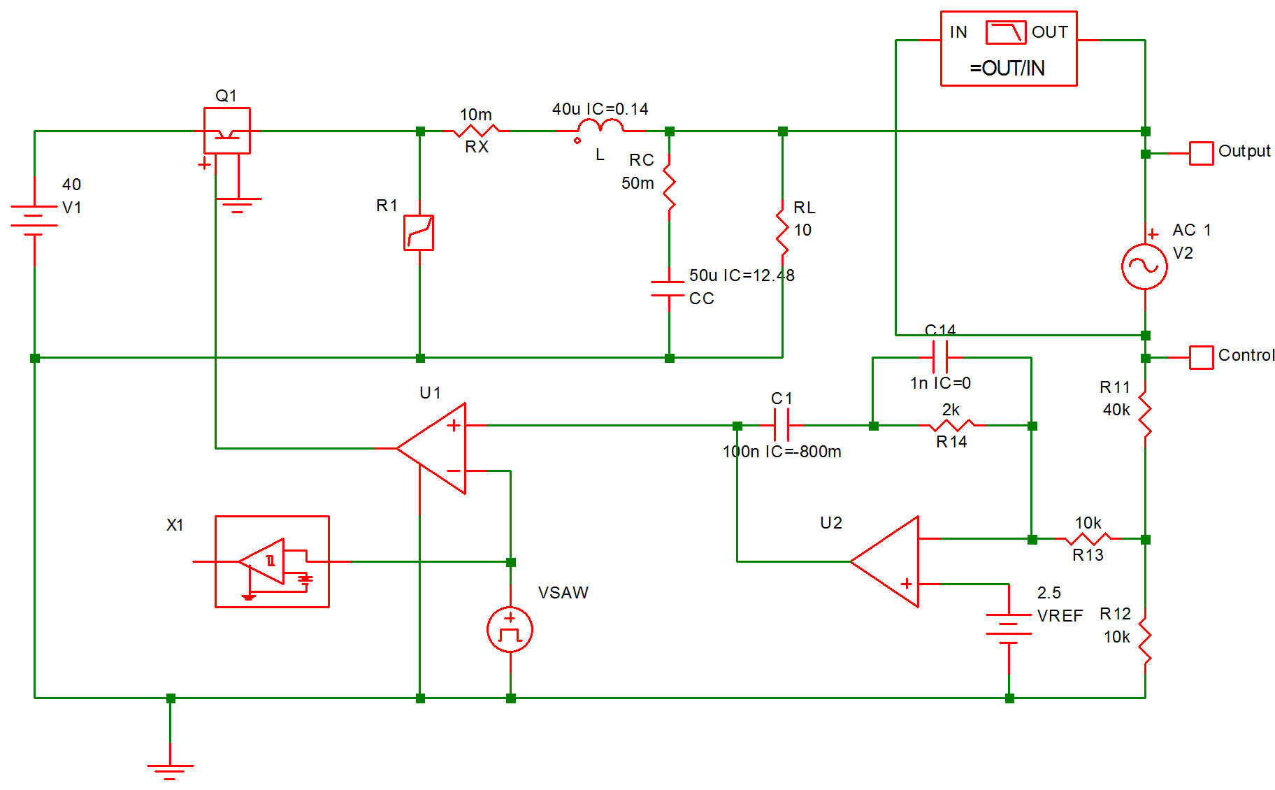 |
11.3 Small-signal excitation to determine the loop gain of the regulated converter. |
Example in User Manual with Small-Signal Analysis
.NODE_MAP Output 15
.NODE_MAP Control 14
.AC DEC 40 1u 50k
.PRINT  ALL
.OPTIONS  PSP_NPT=2001  POP_ITRMAX=40
.POP  TRIG_GATE=X1.!D_CYCLE  TRIG_COND=1_TO_0
+ MAX_PERIOD=50u
X$U2 9 13 8 opamp
VSAW 11 0 SAW V1=0 V2=5 FREQ=100k DELAY=0 OFF_UNTIL_DELAY=NO
X$U1 5 0 9 11 SIMPLIS_COMP$1
V1 2 0 40
V2 15 14 AC 1
VREF 13 0 2.5
L 4 15 40u IC=0.14
R12 0 10 10k
X1 11 12 PERIODIC_OP$2
R13 10 8 10k
RC 6 15 50m
RL 15 0 10
R11 10 14 40k
C1 9 7 100n IC=-800m
R14 8 7 2k
C14 7 8 1n IC=0
CC 6 0 50u IC=12.48
Q1 2 3 5 0 Q1$TP_VCQ IC=OPEN
.MODEL Q1$TP_VCQ VCQPOS VSAT=700m RSAT=100m ROFF=10Meg GAIN=10
+ TH=2.5 HYSTWD=1u LOGIC=POS LEVEL=1
!R$R1 0 3 R1$TP_SSPWLR IC=1
.MODEL R1$TP_SSPWLR VPWLR NSEG=2 X0=0 Y0=0 X1=0.7 Y1=10U
+ X2=0.8 Y2=1.00001
RX 4 3 10m
.SUBCKT PERIODIC_OP$2  1 3
.NODE_MAP IN 1
.NODE_MAP OUT 3
!D_CYCLE 3 0 1 302 M1M IC=1
VREF 302 0 DC 2.5
.MODEL M1M COMP RIN=10MEG ROUT=50 VOL=0 VOH=5
+ HYSTWD=0.001 DELAY=0
.ENDS PERIODIC_OP$2
.SUBCKT SIMPLIS_COMP$1  201 100 101 102
!DCOMP 201 100 101 102 MCOMP IC=1
.MODEL MCOMP COMP RIN=1e+007 ROUT=10 VOL=0 VOH=5
+ HYSTWD=0.1 DELAY=0
.ENDS SIMPLIS_COMP$1
.SUBCKT opamp  2 3 1
.NODE_MAP VINN 1
.NODE_MAP VINP 3
.NODE_MAP VOUT 2
RIN 3 1 5Meg
EOP 2 0 3 1 1Meg
.ENDS opamp
.END
Notice that a small-signal AC source, VSS, is inserted in the feedback loop between the output and control nodes. If the impedance from the control node to ground is much higher than the impedance from the output to ground, the loop gain ???MATH???G(j\omega)???MATH??? of such a regulated system is accurately approximated by the following complex ratio:
\[ G(j\omega) = - Voutput(j\omega)/Vcontrol(j\omega) \]
This is the function of the "Bode Plot Probe" shown at the top right of the schematic 11.3. The result of ???MATH???G(j\omega)???MATH??? for this converter is shown in fig 11.5. In fig 11.5, the gain cross-over occurs at 147 Hz, and the phase margin is about 100 degrees. Although the phase margin is high, indicating the converter is stable as it is, there is room for improvement to this design. The low cross-over frequency means the transient response of this regulated converter would be slow and would take a long time to settle back to the periodic operating equilibrium. Moreover, a zero should be introduced to the loop gain function to compensate for the pair of complex poles at 3.56 kHz which is caused by the output filter formed by L and C. Otherwise, the sharp drop in the phase due to the pair of complex poles can have a very detrimental effect on the stability of the system if the cross-over frequency is pushed higher. Changing the value of R14 will effect the gain cross-over frequency and the phase margin of this converter. As a matter of fact, this converter becomes unstable, with a phase margin of -6 degrees, when the resistor R14 in the feedback loop is raised to ???MATH???16 K\Omega???MATH???!
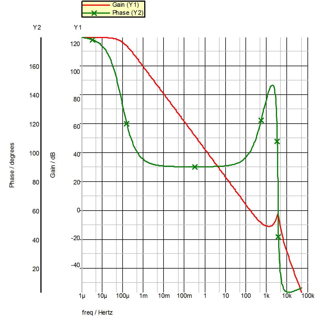 |
11.5 Magnitude and Phase of G(j???MATH???\omega???MATH???). |
| ◄ Statements Relating AC Analysis | Overview ▶ |