Using Expressions
In this topic:
Overview
Expressions consist of arithmetic operators, functions, variables and constants and may be employed in the following locations:
- As device parameters
- As model parameters
- To define a variable (see .PARAM) which can itself be used in an expression.
- As the governing expression used for arbitrary sources.
They have a wide range of uses. For example:
- To define a number of device or model parameters that depend on some common characteristic. This could be a circuit specification such as the cut-off frequency of a filter or maybe a physical characteristic to define a device model.
- To define tolerances used in Monte Carlo analyses.
- Used with an arbitrary source, to define a non-linear device.
Using Expressions for Device Parameters
Device or instance parameters are placed on the device line. For example the length parameter of a MOSFET, L, is a device parameter. A MOSFET line with constant parameters might be:
M1 1 2 3 4 MOS1 L=1u W=2u
L and W could be replaced by expressions. For example:
M1 1 2 3 4 MOS1 L={LL-2*EDGE} W={WW-2*EDGE}
Device parameter expressions must usually be enclosed with either single quotation marks ( ' ) double quotation marks ( " ) or braces ( '{' and '}' ). The expression need not be so enclosed if it consists of a single variable. For example:
.PARAM LL=2u WW=1u
M1 1 2 3 4 MOS1 L=LL W=WW
Using Expressions for Model Parameters
The rules for using expressions for device parameters also apply to model parameters. E.g.
.MODEL N1 NPN IS=is BF={beta*1.3}
Expression Syntax
Expressions generally comprise the following elements:
- Circuit variables
- Parameters
- Constants.
- Operators
- Functions
- Look up tables
Circuit Variables
Circuit variables may only be used in expressions used to define arbitrary sources and to define variables that themselves are accessed only in arbitrary source expressions.
Circuit variables allow an expression to reference voltages and currents in any part of the circuit being simulated.
Voltages are of the form:
V(node_name1)
V(node_name1, node_name2)
Where node_name1 and node_name2 are the name of the node carrying the voltage of interest. The second form above returns the difference between the voltages on node_name1 and node_name2. If using the schematic editor nodenames are normally allocated by the netlist generator. For information on how to display and edit the schematic's node names, refer to Displaying Net and Pin Names.
Currents are of the form:
I(source_name)
Where source_name is the name of a voltage source carrying the current of interest. The source may be a fixed voltage source, a current controlled voltage source, a voltage controlled voltage source or an arbitrary voltage source. It is legal for an expression used in an arbitrary source to reference itself e.g.:
B1 n1 n2 V=100*I(B1)
Implements a 100 ohm resistor.
Parameters
These are defined using the .PARAM statement. For example:
.PARAM res=100
B1 n1 n2 V=res*I(B1)
Also implements a 100 ohm resistor.
Circuit variables may be used .PARAM statements, for example:
.PARAM VMult = { V(a) * V(b) }
B1 1 2 V = Vmult + V(c)
Parameters that use circuit variables may only be used in places where circuit variables themselves are allowed. So, they can be used in arbitrary sources and they may be used to define the resistance of an Hspice style resistor which allows voltage and current dependence. (See Resistor - Hspice Compatible). They may also of course be used to define further parameters as long as they too comply with the above condition.
Built-in Parameters
A number of parameter names are assigned by the simulator. These are:
| Parameter name | Description |
| TIME | Resolves to time for transient analysis. Resolves to 0 otherwise including during the pseudo transient operation point algorithm. Note that this may only be used in an arbitrary source expression |
| TEMP | Resolves to current circuit temperature in Celsius |
| HERTZ | Resolves to frequency during AC sweep and zero in other analysis modes |
| PTARAMP | Resolves to value of ramp during pseudo transient operating point algorithm if used in arbitrary source expression. Otherwise this value resolves to 1. |
Constants
Apart from simple numeric values, arbitrary expressions may also contain the following built-in constants:
| Constant name | Value | Description |
| PI | 3.14159265358979323846 | ???MATH???\pi???MATH??? |
| E | 2.71828182845904523536 | e |
| TRUE | 1.0 | |
| FALSE | 0.0 | |
| ECHARGE | 1.6021918e-19 | Charge on an electron in coulombs |
| BOLTZ | 1.3806226e-23 | Boltzmann's constant |
B1 n1 n2 V = V(n3, n3) * { global:amp_gain }
amp_gain could be defined in a script using the LET command. E.g. "Let global:amp_gain = 100"
Operators
These are listed below and are listed in order of precedence. Precedence controls the order of evaluation. So 3*4 + 5*6 = (3*4) + (5*6) = 42 and 3+4*5+6 = 3 + (4*5) + 6 = 29 as '*' has higher precedence than '+'.
| Operator | Description |
| ~ ! - | Digital NOT, Logical NOT, Unary minus |
| ^ or ** | Raise to power. |
| *, / | Multiply, divide |
| +, - | Plus, minus |
| >=, <=, > < | Comparison operators |
| ==, != or <> | Equal, not equal |
| & | Digital AND (see below) |
| | | Digital OR (see below) |
| && | Logical AND |
| ^^ | Exclusive OR |
| || | Logical OR |
| test ? true_expr : false_expr | Ternary conditional expression (see below) |
Comparison, Equality and Logical Operators
These are Boolean in nature either accepting or returning Boolean values or both. A Boolean value is either TRUE or FALSE. FALSE is defined as equal to zero and TRUE is defined as not equal to zero. So, the comparison and equality operators return 1.0 if the result of the operation is true otherwise they return 0.0.
The arguments to equality operators should always be expressions that can be guaranteed to have an exact value e.g. a Boolean expression or the return value from functions such as SGN. The == operator, for example, will return TRUE only if both arguments are exactly equal. So the following should never be used:
v(n1)==5.0
v(n1) may not ever be exactly 5.0. It may be 4.9999999999 or 5.00000000001 but only by chance will it be 5.0.
These operators are intended to be used with the IF() function described in Ternary Conditional Expression.
Digital Operators
These are the operators '&', '|' and '~'. These were introduced in old SIMetrix version as a simple means of implementing digital gates in the analog domain. Their function has largely been superseded by gates in the event driven simulator but they are nevertheless still supported.
Although they are used in a digital manner the functions implemented by these operators are continuous in nature. They are defined as follows:
| Expression | Condition | Result |
| out = x & y | x<vtl OR y<vtl | out = vl |
| x>vth AND y>vth | out = vh | |
| x>vth AND vth>y>vtl | out = (y-vtl)*(vh-vl)/(vth-vtl)+vl | |
| vtl<x< vth AND y>vth | out = (x-vtl)*(vh-vl)/(vth-vtl)+vl | |
| vtl<x< vth AND vth>y>vtl | out = (y-vtl)*(x-vtl)*(vh-vl)/(vth-vtl)2+vl | |
| out = x|y | x<vtl AND y<vtl | out = vl |
| x>vth OR y>vth | out = vh | |
| x<vtl AND vth>y>vtl | out = vh-(vth-y)*(vh-vl)/(vth-vtl) | |
| vtl<x< vth AND y<vtl | out = vh-(vth-x)*(vh-vl)/(vth-vtl) | |
| vtl<x< vth AND vth>y>vtl | out = vh-(vth-y)*(vth-x)*(vh-vl)/(vth-vtl)2 | |
| out = ~ x | x<vtl | out = vh |
| x>vth | out = vl | |
| vtl<x< vth | out = (vth-x)/(vth-vtl)*(vh-vl)+vl |
Where:
- vth = upper input threshold
- vtl = lower input threshold
- vh = output high
- vl = output low
- LOGICTHRESHHIGH,
- LOGICTHRESHLOW,
- LOGICHIGH,
- LOGICLW
To change the lower input threshold to 1.9, add the following line to the netlist:
.OPTIONS LOGICTHRESHLOW=1.9
To find out how to add additional lines to the netlist when using the schematic editor, refer to Adding Extra Netlist Lines.
Ternary Conditional Expression
This is of the form:
test_expression ? true_expression : false_expression
The value returned will be true_expression if test_expression resolves to a non-zero value, otherwise the return value will be false_expression. This is functionally the same as the IF() function described in the functions table below.
Functions
| Function | Description |
| ABS(x) | ???MATH???|x|???MATH??? |
| ACOS(x), ARCCOS(x) | ???MATH???cos^{-1}(x)???MATH??? |
| ACOSH(x) | ???MATH???cosh^{-1}(x)???MATH??? |
| ASIN(x), ARCSIN(x) | ???MATH???sin^{-1}(x)???MATH??? |
| ASINH(x) | ???MATH???sinh^{-1}(x)???MATH??? |
| ATAN(x), ARCTAN(x) | ???MATH???tan^{-1}(x)???MATH??? |
| ATAN2(x,y) | ???MATH???tan^{-1}(x/y)???MATH???. Valid if y=0 |
| ATANH(x) | ???MATH???tanh^{-1}(x)???MATH??? |
| COS(x) | ???MATH???cos(x)???MATH??? |
| COSH(x) | ???MATH???cosh(x)???MATH??? |
| DDT(x) | ???MATH???dx/dt???MATH??? |
| EXP(x) | ???MATH???e^{x}???MATH??? |
| FLOOR(x), INT(x) | Next lowest integer of ???MATH???x???MATH???. |
| IF(cond, x, y[, maxslew]) | if cond is TRUE ???MATH???result=x???MATH??? else ???MATH???result=y???MATH???. If ???MATH???maxslew>0???MATH??? the rate of change of the result will be slew rate controlled. See IF() Function. |
| IFF(cond, x, y[, maxslew]) | As IF(cond, x, y, maxslew) |
| LIMIT(x, lo, hi) | if ???MATH???x<lo???MATH??? ???MATH???result=lo???MATH??? else if ???MATH???x>hi???MATH??? ???MATH???result=hi???MATH??? else ???MATH???result=x???MATH??? |
| LIMITS(x, lo, hi, sharp) | As LIMIT but with smoothed corners. The 'sharp' parameter defines the abruptness of the transition. A higher number gives a sharper response. LIMITS gives better convergence than LIMIT. See LIMITS() Function. below |
| LN(x) | ???MATH???ln(x)???MATH??? If ???MATH???x<10^{-100}???MATH??? ???MATH???result=-230.2585093???MATH??? |
| LNCOSH(x) | ???MATH???ln(cosh(x))???MATH??? = ???MATH???\int tanh(x) dx???MATH??? |
| LOG(x) | ???MATH???log_{10}(x)???MATH???. If ???MATH???x<10^{-100}???MATH??? ???MATH???result=-100???MATH??? |
| LOG10(x) | ???MATH???log_{10}(x)???MATH???. If ???MATH???x<10^{-100}???MATH??? ???MATH???result=-100???MATH??? |
| MAX(x, y) | Returns larger of ???MATH???x???MATH??? and ???MATH???y???MATH??? |
| MIN(x,y) | Returns smaller of ???MATH???x???MATH??? and ???MATH???y???MATH??? |
| PWR(x,y) | ???MATH???x^y???MATH??? |
| PWRS(x,y) | ???MATH???x>=0???MATH???: ???MATH???x^y???MATH???, ???MATH???x<0???MATH???: ???MATH???-x^y???MATH??? |
| SDT(x) | ???MATH???\int x dt???MATH??? |
| SGN(X) | ???MATH???x>0???MATH???: 1, ???MATH???x<0???MATH???: -1, ???MATH???x=0???MATH???: 0 |
| SIN(x) | ???MATH???sin(x)???MATH??? |
| SINH(x) | ???MATH???sinh(x)???MATH??? |
| SQRT(x) | ???MATH???x>=0???MATH???: ???MATH???\sqrt{x}???MATH???, ???MATH???x<0???MATH???: ???MATH???\sqrt{-x}???MATH??? |
| STP(x) | ???MATH???x<=0???MATH???: 0, ???MATH???x>0???MATH???: 1 |
| TABLE(x,xy_pairs) | lookup table. Refer to Lookup tables |
| TABLEX(x,xy_pairs) | Same as TABLE except end points extrapolated. Refer to Lookup tables |
| TAN(x) | ???MATH???tan(x)???MATH??? |
| TANH(x) | ???MATH???tanh(x)???MATH??? |
| U(x) | as STP(x) |
| URAMP(x) | ???MATH???x<0???MATH???: 0, ???MATH???x>=0???MATH???: ???MATH???x???MATH??? |
Monte Carlo Distribution Functions
To specify Monte Carlo tolerance for a model parameter, use an expression containing one of the following functions:
| Name | Distribution | Lot? |
| DISTRIBUTION | User defined distribution | No |
| DISTRIBUTIONL | User defined distribution | Yes |
| UD | Alias for DISTRIBUTION() | No |
| UDL | Alias for DISTRIBUTIONL() | Yes |
| GAUSS | Gaussian | No |
| GAUSSL | Gaussian | Yes |
| GAUSSTRUNC | Truncated Gaussian | No |
| GAUSSTRUNCL | Truncated Gaussian | Yes |
| UNIF | Uniform | No |
| UNIFL | Uniform | Yes |
| UNIF2 | Uniform | No |
| UNIFL2 | Uniform | Yes |
| WC | Worst case | No |
| WCL | Worst case | Yes |
| WC2 | Worst case | No |
| WCL2 | Worst case | Yes |
| GAUSSE | Gaussian logarithmic | No |
| GAUSSEL | Gaussian logarithmic | Yes |
| UNIFE | Uniform logarithmic | No |
| UNIFEL | Uniform logarithmic | Yes |
| WCE | Worst case logarithmic | No |
| WCEL | Worst case logarithmic | Yes |
IF() Function
IF(condition, true-value, false-value[, max-slew])The result is:
if condition is non-zero, result is true-value, else result is false-value.
If max-slew is present and greater than zero, the result will be slew-rate limited in both positive and negative directions to the value of max-slew.
In some situations, for example if true-value and false-value are constants, the result of this function will be discontinuous when condition changes state. This can lead to non-convergence as there is no lower bound on the time-step. In these cases a max-slew parameter can be included. This will limit the slew rate so providing a controlled transition from the true-value to the false-value and vice-versa.
If the option setting DISCONTINUOUSIFSLEWRATE is non-zero, SIMetrix will automatically apply a max-slew parameter to all occurrences of the IF() function if both true-value and false-value are constants. This provides a convenient way of resolving convergence issues with third-party models that make extensive use of discontinuous if expressions. Note that the DISCONTINUOUSIFSLEWRATE option is also applied to conditional expressions using the C-style condition ? true-value : false-value syntax.
LIMITS() Function
LIMITS(x, low, high, sharp)The LIMITS() function is similar to LIMIT but provides a smooth response at the corners which leads to better convergence behaviour. The behaviour is shown below
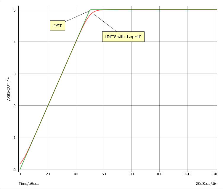
The LIMITS function follows this equation:
LIMITS(x, low, high, sharp) = 0.5*((ln(cosh(v1))-ln(cosh(v2)))/v3 +(low+high))
- v1 = sharp/(high-low)*(x-low)
- v2 = sharp/(high-low)*(x-high)
- v3 = sharp/(high-low)
Look-up Tables
| Method 1 |
Syntax in form: TABLE[xy_pairs](input_expression).
|
||||
| Method 2 |
Syntax in form: TABLE(input_expression, xy_pairs).
|
||||
| Method 3 |
Syntax in form: TABLEX(input_expression, xy_pairs).
|
Method 1 is more efficient at handling large tables (hundreds of values). However, method 2 is generally more flexible and is the recommended choice for most applications. Method 2 is also compatible with other simulators whereas method 1 is proprietary to SIMetrix.
For an example see Table Lookup Example
Examples
Table Lookup Example
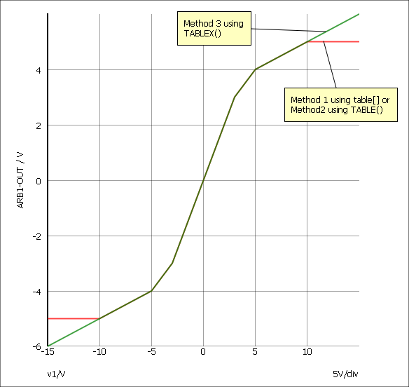
The following arbitrary source definition implements a soft limiting function
B1 n2 n3 V=table[-10, -5, -5, -4, -4, -3.5, -3, -3, 3, 3, 4,
+ 3.5, 5, 4, 10, 5](v(N1))
B1 n2 n3 V=TABLE(v(N1), -10, -5, -5, -4, -4, -3.5, -3, -3, 3, 3, 4,
+ 3.5, 5, 4, 10, 5)
B1 n2 n3 V=TABLEX(v(N1), -10, -5, -5, -4, -4, -3.5, -3, -3, 3, 3, 4,
+ 3.5, 5, 4, 10, 5)
The resulting transfer functions are illustrated in the following picture:
Parameter Example
It is possible to assign expressions to component values which are evaluated when the circuit is simulated. This has a number of uses. For example you might have a filter design for which several component values affect the roll off frequency. Rather than recalculate and change each component every time you wish to change the roll of frequency it is possible to enter the formula for the component's value in terms of this frequency.
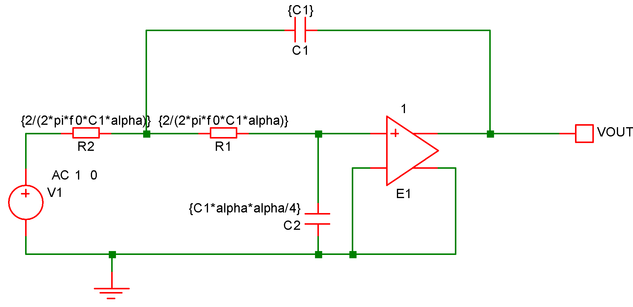
The above circuit is that of a two pole low-pass filter. C1 is fixed and R1=R2. The design equations are:
R1=R2=2/(2*pi*f0*C1*alpha)
C2=C1*alpha*alpha/4
where f0 is the cut off frequency and alpha is the damping factor.
The complete netlist for the above circuit is:
V1 V1_P 0 AC 1 0
C2 0 R1_P {C1*alpha*alpha/4}
C1 VOUT R1_N {C1}
E1 VOUT 0 R1_P 0 1
R1 R1_P R1_N {2/(2*pi*f0*C1*alpha)}
R2 R1_N V1_P {2/(2*pi*f0*C1*alpha)}
Before running the above circuit you must assign values to the variables. This can be done by one of three methods:
- With the .PARAM statement placed in the netlist.
- With Let command from the command line or from a script. (If using a script you must prefix the parameter names with global:)
- By sweeping the value with using parameter mode of a swept analysis (see General Sweep Specification) or multi-step analysis (see Multi Step Analyses).
Suppose we wish a 1kHz roll off for the above filter.
Using the .PARAM statement, add these lines to the netlist
.PARAM f0 1k
.PARAM alpha 1
.PARAM C1 10n
Using the Let command, you would type:
Let f0=1k
Let alpha=1
Let C1=10n
Let alpha=0.8
then re-run the simulator.
To execute the Let commands from within a script, prefix the parameter names with global:. E.g. "Let global:f0=1k"
In many cases the .PARAM approach is more convenient as the values can be stored with the schematic.
Optimisation
Overview
An optimisation algorithm may be enabled for expressions used to define arbitrary sources and any expression containing a swept parameter. This can improve performance if a large number of such expressions are present in a design.
The optimiser dramatically improves the simulation performance of the power device models developed by Infineon. See Optimiser Performance.
Why is it Needed?
The simulator's core algorithms use the Newton-Raphson iteration method to solve non-linear equations. This method requires the differential of each equation to be calculated and for arbitrary sources, this differentiation is performed symbolically. So as well as calculating the user supplied expression, the simulator must also evaluate the expression's differential with respect to each dependent variable. These differential expressions nearly always have some sub-expressions in common with sub-expressions in the main equation and other differentials. Calculation speed can be improved by arranging to evaluate these sub-expressions only once. This is the main task performed by the optimiser. However, it also eliminates factors found on both the numerator and denominator of an expression as well as collecting constants together wherever possible.
Using the Optimiser
The optimiser is automatically enabled and no action is required to make use of it. If desired, it can be disabled using:
.OPTIONS optimise=0
Optimiser Performance
The optimisation algorithm was added to SIMetrix primarily to improve the performance of some publicly available power device models from Infineon. These models make extensive use of arbitrary sources and many expressions are defined using .FUNC.
The performance improvement gained for these model is in some cases dramatic. For example a simple switching PSU circuit using a SGP02N60 IGBT ran around 5 times faster with the optimiser enabled and there are other devices that show an even bigger improvement.
Accuracy
The optimiser simply changes the efficiency of evaluation and doesn't change the calculation being performed in any way. However, performing a calculation in a different order can alter the least significant digits in the final result. In some simulations, these tiny changes can result in much larger changes in circuit solution. So, you may find that switching the optimiser on and off may change the results slightly.
| ◄ Using XSPICE Devices | Subcircuits ▶ |