Specifying Tolerances
In this topic:
Overview
Tolerances for Monte Carlo analysis may be specified by one of the following methods:
- Using a distribution function in an expression.
- Using the device parameters TOL, MATCH and LOT
Distribution Functions
To specify Monte Carlo tolerance for a model or device parameter, define the parameter using an expression (see Using Expressions) containing one of the following functions:
| Name | Distribution | Lot? |
| GAUSS(tol) | Gaussian (3-sigma) | No |
| GAUSSL(tol) | Gaussian (3-sigma) | Yes |
| UNIF(tol) | Uniform | No |
| UNIFL(tol) | Uniform | Yes |
| UNIF2(tolupper, tollower) | Uniform | No |
| UNIFL2(tolupper, tollower) | Uniform | Yes |
| WC(tol) | Worst case | No |
| WCL(tol) | Worst case | Yes |
| WC2(tolupper, tollower) | Worst case | No |
| WCL2(tolupper, tollower) | Worst case | Yes |
| GAUSSTRUNC(tol, sigma) | Truncated Gaussian | No |
| GAUSSTRUNCL(tol, sigma) | Truncated Gaussian | Yes |
| DISTRIBUTION(args) | User defined distribution | No |
| DISTRIBUTIONL(args) | User defined distribution | Yes |
| UD(args) | User defined distribution (alias) | No |
| UDL(args) | User defined distribution (alias) | Yes |
Each of the above functions takes a single argument that specifies the tolerance. The return value is 1.0 +/- tolerance with the exception of GAUSS and GAUSSL. See Gaussian Distributions for details. In non-Monte Carlo analyses, all of the above return unity.
The graphs below show the characteristics of the various distributions. The curves were plotted by performing an actual Monte Carlo run with 100000 steps.
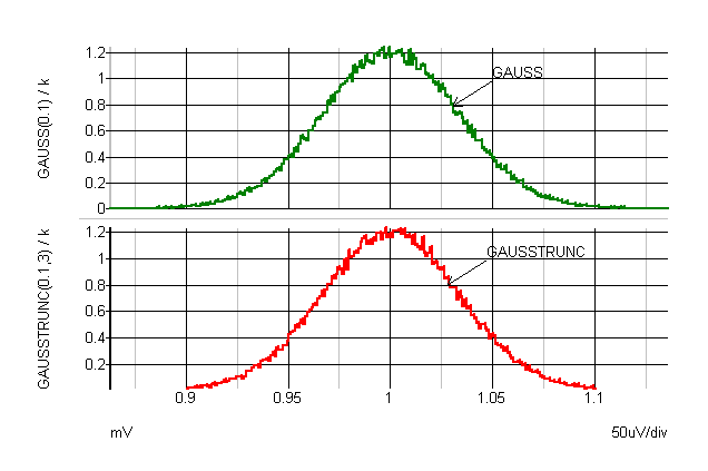 |
GAUSS and GAUSSTRUNC |
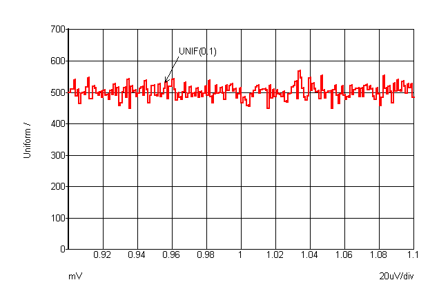 |
UNIF |
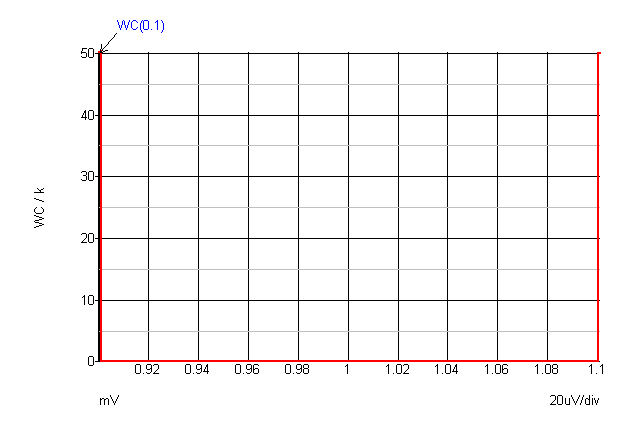 |
WC |
User Defined Distribution
Customised distributions may be defined using the Distribution function (or its alias UD).
| Arg | Desription |
| 1 | Base tolerance. In effect scales the extent of the distribution defined in the remaining arguments |
| Remaining arguments | Lookup table organised in pairs of values. The first value in the pair is the deviation. This should be in the range +1 to -1 and maps to the output range. So +1 corresponds to an output value of +tolerance and -1 corresponds to -tolerance. Each deviation value must be greater than or equal to the previous value. Values outside the range +/- 1 are allowed but will result in the function being able to return values outside the tolerance range. The second value in the pair is the relative probability and must 0 or greater. There is no limit to the number of entries in the table |
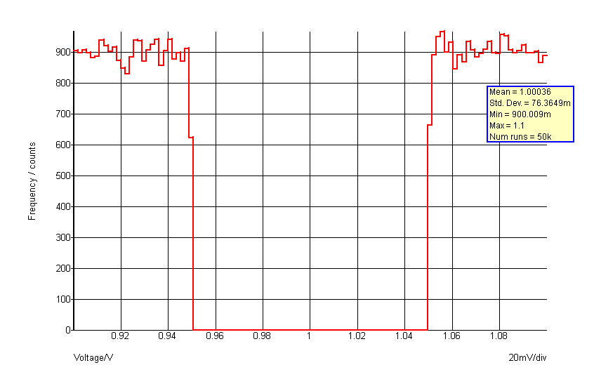
Custom distributions can be conveniently defined using the .FUNC function definition statement. For example, the following defines a binomial distribution:
.FUNC binomial(a) = {distribution(a, -1,1, -0.5,1, -0.5,0, 0.5,0, 0.5,1, 1,1 )}
The function 'binomial()' can subsequently be used in the same way as other distribution functions. This would have a distribution as shown in the following graph:
Gaussian Distributions
The standard Gaussian distribution functions (GAUSS(), GAUSSL()) return a random variable with a true Gaussian distribution where the tolerance value represents the 3???MATH???\sigma???MATH??? spread. This can return values that are outside the tolerance specification albeit with low probability. For example GAUSS(0.1) can return values >1.1 and less than 0.9 as defined by the Gaussian distribution. For specifying actual components this is not usually exactly correct as most components are tested at production and devices outside the specified tolerance will be rejected.
This type of component can instead be specified using the GAUSSTRUNC() distibution function. This rejects values outside the specified range expressed as a multiple of ???MATH???\sigma???MATH???. Syntax for the GAUSSTRUNC() function is:
GAUSSTRUNC(tolerance, sigma_multiplier)
Where:
| Arg | Desription |
| tolerance | Tolerance. Return value will lie in range 1.0 +/- tolerance |
| sigma_multiplier | Standard deviation of output expressed as multiplier of ???MATH???\sigma???MATH??? |
Examples
Apply 50% tolerance to BF parameter of BJT with gaussian distribution.
.MODEL NPN1 NPN IS=1.5e-15 BF={180*GAUSS(0.5)}
R1 n1 n2 {4.7K*GAUSSTRUNC(0.1,3)}
Lot Tolerances
The lot versions of the functions specify a distribution to be applied to devices whose tolerances track. These functions will return the same random value for all devices that reference the same model.
Note that the same effect as LOT tolerances can be achieved using random variables and subcircuits. For details see Creating Random Variables
Lot Tolerance Examples
Specify 50% uniform lot tolerance and 5% gaussian device tolerance for BF parameter
.MODEL NPN1 NPN IS=1.5E-15 BF={180*GAUSS(0.05)*UNIFL(0.5)}
Here is an abbreviated log file for a run of a circuit using 2 devices referring to the above model:
Run 1                    Run 2
Device    Nom.      Value      (Dev.)        Value     (Dev.)
Q1:bf     180     93.308486 (-48.162% )    241.3287  (34.0715% )
Q2:bf     180     91.173893 (-49.3478%)    245.09026 (36.16126%)

Run 3                    Run 4
Device    Nom.      Value      (Dev.)        Value     (Dev.)
Q1:bf     180     185.95824 (3.310133%)    210.46439 (16.92466%)
Q2:bf     180     190.8509  (6.02828% )    207.04202 (15.02335%)
For the four runs BF varies from 91 to 245 but the two devices never deviate from each other by more than about 2.7%.
Notes
The tracking behaviour may not be as expected if the model definition resides within a subcircuit. When a model is defined in a subcircuit, a copy of that model is created for each device that calls the subcircuit. Here is an example:
XQ100 VCC INN Q100_E 0 NPN1
XQ101 VCC INP Q101_E 0 NPN1

.SUBCKT NPN1 1 2 3 SUB
Q1 1 2 3 SUB N1
Q2 SUB 1 2 SUB P1

.MODEL N1 NPN IS=1.5E-15 BF={180*GAUSS(0.05)*UNIFL(0.5)}
.ENDS
In the above, XQ100 and XQ101 will not track. Two devices referring to N1 inside the subcircuit definition would track each other but different instances of the subcircuit will not. To make XQ100 and XQ101 track, the definition of N1 should be placed outside the subcircuit. E.g.
XQ100 VCC INN Q100_E 0 NPN1
XQ101 VCC INP Q101_E 0 NPN1

.SUBCKT NPN1 1 2 3 SUB
Q1 1 2 3 SUB N1
Q2 SUB 1 2 SUB P1

.ENDS
.MODEL N1 NPN IS=1.5E-15 BF={180*GAUSS(0.05)*UNIFL(0.5)}
Creating Random Variables
It is possible to place distribution functions in .PARAM expressions to create a random variable. This provides a means of describing a relationship between different devices or different parameters within the same device.
Random variables may be created at the top level in which case they will be global and have the same value wherever they are used. Random variables may also be created inside subcircuit definitions. In this case they are local to the subcircuit and will have the same value for all devices and parameters within the subcircuit but a different value for different instances of the subcircuit.
Example 1 In this example we make a BJT model using a subcircuit. The random variable is created inside the subcircuit so will have the same value for parameters defined in the subcircuit but will have different values for multiple instances
.subckt NPN1 c b e
.PARAM rv1 = UNIF(0.5)
Q1 c b e NPN1
.MODEL NPN1 NPN BF={rv1*180} TF={1e-11*rv1}
.ends
For all devices using that model, BF and TF will always have a fixed relationship to each other even though each parameter can vary by +/-50% from one device to the next.
Here is the log of a run carried out on a circuit with two of the above devices:
Run 1                    Run 2
Run 1: Seed=1651893287

Run 1
Device    Nom.         Value        (Dev.)
Q1.Q1:bf 180          148.83033746 (-17.3164792%)
Q1.Q1:tf 10p          8.268352081p (-17.3164792%)
Q2.Q1:bf 180          129.69395145 (-27.9478048%)
Q2.Q1:tf 10p          7.205219525p (-27.9478048%)

Run 2: Seed=763313972

Run 2
Device    Nom.         Value        (Dev.)
Q1.Q1:bf 180          265.86053442 (47.7002969% )
Q1.Q1:tf 10p          14.77002969p (47.7002969% )
Q2.Q1:bf 180          186.41647487 (3.564708261%)
Q2.Q1:tf 10p          10.35647083p (3.564708261%)
Notice that the BF and TF parameters always deviate by exactly the same amount for each device. However, the two devices do not track each other. If this were needed we would define the random variable outside the subcircuit at the netlist's top level:
.PARAM rv1 = UNIF(0.5)
.subckt NPN1 c b e
Q1 c b e NPN1
.MODEL NPN1 NPN BF={rv1*180} TF={1e-11*rv1}
.ends
Here is the log for the above:
Run 1: Seed=1608521901

Run 1
Device    Nom.         Value        (Dev.)
Q1.Q1:bf 180          249.54358268 (38.63532371%)
Q1.Q1:tf 10p          13.86353237p (38.63532371%)
Q2.Q1:bf 180          249.54358268 (38.63532371%)
Q2.Q1:tf 10p          13.86353237p (38.63532371%)

Run 2: Seed=80260241

Run 2
Device    Nom.         Value        (Dev.)
Q1.Q1:bf 180          116.33087232 (-35.3717376%)
Q1.Q1:tf 10p          6.46282624p  (-35.3717376%)
Q2.Q1:bf 180          116.33087232 (-35.3717376%)
Q2.Q1:tf 10p          6.46282624p  (-35.3717376%)
Hspice Distribution Functions
SIMetrix supports the Hspice method of defining Monte Carlo tolerances. This feature needs to be enabled with an option setting; see Enabling Hspice Distribution Functions. The Hspice method uses random variables created using a special .PARAM syntax in one of the following form:
.PARAM parameter_name [=] AGAUSS(nominal, abs_variation, sigma, [multiplier]) ...
.PARAM parameter_name [=] AUNIF(nominal, abs_variation, [multiplier]) ...
.PARAM parameter_name [=] GAUSS(nominal, rel_variation, sigma, [multiplier]) ...
.PARAM parameter_name [=] UNIF(nominal, rel_variation, [multiplier]) ...
| parameter_name | Name of random variable |
| nominal | Nominal value |
| abs_variation | Absolute variation. AGAUSS and AUNIF vary the nominal value +/- this value |
| rel_variation | Relative variation. GAUSS and UNIF vary the nominal value by +/- rel_variation*nominal |
| sigma | Scales abs_variation and rel_variation for functions GAUSS and AGAUSS. E.g. if sigma is 3 the standard deviation of the result is divided by 3. So AGAUSS(0,0.01,3) would yield a +/-1% tolerance with a 3 sigma distribution |
| multiplier | If included this must be set to 1 otherwise an error message will be displayed and the simulation aborted. Included for compatibility with existing model files only. |
For example, the following are both quite legal:
.PARAM rv1 = UNIF(10,1)
.PARAM rv2 = 'UNIF(10,1)'
The first (rv1) will provide a nominal value 10.0 +/- 1.0 with a new value calculated each time it is used. The second (rv2) is a native SIMetrix distribution function, will produce a value varying from -9.0 to +11.0 and will always have the same value. With the above definitions for rv1 and rv2, consider the following regular .PARAM statements:
.PARAM rand1 = rv1
.PARAM rand2 = rv1
.PARAM rand3 = rv2
.PARAM rand4 = rv2
rand1 and rand2 will have different values. rand3 and rand4 will have the same values.
Enabling Hspice Distribution Functions
Hspice distribution functions need to be enabled with an option setting as follows:
.OPTIONS MCHSPICE
Important: This option also changes the way Monte Carlo operates in a fundamental way by disabling model spawning. This is a process which gives each instance its own separate copy of its model parameters and allows 'dev' (or 'mismatch') tolerances to be implemented. Without model spawning dev tolerances cannot be implemented except by giving every instance their own copy of a model.
With the Hspice method this can only be done easily by wrapping up .MODEL statements inside a .SUBCKT definition. Each instance will then effectively get its own .MODEL statement and mismatch parameters can be defined.
TOL, MATCH and LOT Device Parameters
These parameters may be used as a simple method of applying tolerances to simple devices such as resistors. The TOL parameter specifies the tolerance of the device's value. E.g.
R1 1 2 1K TOL=0.05
The above resistor will have a tolerance of 5% with a gaussian distribution by default. This can be changed to a uniform distribution by setting including the line:
.OPTIONS MC_ABSOLUTE_RECT
in the netlist.
Multiple devices can be made to track by specifying a LOT parameter. Devices with the same LOT name will track. E.g.
R1 1 2 1K TOL=0.05 LOT=RES1
R2 3 4 1k TOL=0.05 LOT=RES1
R1 and R2 in the above will always have the same value.
Deviation between tracking devices can be implemented using the MATCH parameter. E.g.
R1 1 2 1K TOL=0.05 LOT=RES1 MATCH=0.001
R2 3 4 1k TOL=0.05 LOT=RES1 MATCH=0.001
R1 and R2 will have a tolerance of 5% but will always match each other to 0.1%. MATCH tolerances are gaussian by default but can be changed to uniform by specifying
.OPTIONS MC_MATCH_RECT
The default distributions for tolerances defined this way are the logarithmic versions as described in Distribution Functions. To use a linear distribution, add this statement to netlist (or F11 window in the schematic editor):
.OPTIONS mcUseLinearDistribution
If using device tolerance parameters, note that any absolute tolerance specified must be the same for all devices within the same lot. Any devices with the same lot name but different absolute tolerance will be treated as belonging to a different lot. For example if a circuit has four resistors all with lot name RN1 but two of them have an absolute tolerance of 1% and the other two have an absolute tolerance of 2%, the 1% devices won't be matched to the 2% devices. The 1% devices will however be matched to each other as will the 2% devices. This does not apply to match tolerances. It's perfectly OK to have devices with different match tolerances within the same lot.
| ◄ Seeding the Random Number Generator | Overview ▶ |