Laplace Transfer Function - Convolution Implementation
In this topic:
Netlist Entry
Uxxxx p n cp cn modelname [M=m IC=ic VOLTAGE_MODE=vm]
| p | Positive output |
| n | Negative output |
| cp | Positive control input |
| cn | Negative control input |
| modelname | Name of model defined in a .MODEL statement. Must begin with a letter but can contain any character except whitespace and period '.'. |
| ic | Initial condition. If specified, the output will be fixed at this value when the DC operating point is being calculated. If not specified, the device will behave like a fixed gain block with a gain set by the Laplace transfer function with s=0. |
Model Syntax
.model modelname LAPLACE ( parameters )
Model Parameters
| Name | Description | Units | Default |
| EXPR | Laplace transfer function | n/a | |
| DELAY | Additional delay | s | 0 |
| CONV_N | ???MATH???\log_2???MATH???(convolution size) | 15 | |
| DCGAIN | DC gain of block | Note 1 | |
| IMPULSE_METHOD | Method to extract impulse response 0: Use all methods 1: Analytical only 2: Inverse FFT 3: Stehfest | 0 | |
| IMPULSE_TEST_TOL | Impulse response test tolerance | 0.1 | |
| IMPULSE_TEST_FMAX | Maximum test frequency as multiple of 1/TSTOP | 256 | |
| IMPULSE_TEST_FMIN | Minimum test frequency as multiple of 1/TSTOP | 8 | |
| IMPULSE_IFFT_N | ???MATH???\log_2???MATH???(Inverse FFT size) | 20 | |
| IMPULSE_IFFT_TEST_METHOD | Test method for inverse FFT. 0: Spot frequency 1: Zero tail | 1 | |
| TRUNC_TEST | Enable truncation error test | 1 | |
| TRUNC_RELTOL | Truncation error test relative tolerance | 0.05 | |
| TRUNC_ABSTOL | Truncation error test absolute tolerance | 1e-6 | |
| IMPULSE_ENABLE_CACHE | Enable impulse response cache | 1 | |
| PSPICE_COMPAT | Enable PSpice compatibility | 0 | |
| TABLE_ZERO_FREQ | F=0 frequency in table | Hz | Note 2 |
| TABLE_ZERO_MAG | Magnitude=0 in table | 1e-30 | |
| FREQUENCY_SCALE | Substitutes s with s/frequency_scale | 1 | |
| IMPULSE_ENABLE_DIAGNOSTICS | Enable impulse response diagnostics | 0 |
| Note 1 | Gain of block defaults to the value of the Laplace transfer function with s=0. If the transfer function cannot be evaluated at s=0, the expression is evaluated with s=1e-11. If that also fails DCGAIN is set to zero |
| Note 2 | If PSPICE_COMPAT=0 1e-30 otherwise 1e-305 |
Laplace transfer function
The Laplace expression defines the behaviour of the device in the frequency domain. For example '1/(s+1)', defines a simple single pole low-pass filter. The expression may contain arithmetic operators and a number of functions as described in the following sections. Be aware that not any expression is physically realisable; for example 'exp(s)' defines a negative delay, that is a device whose output responds to an input in the future.
Operators
+ - * / ^where \^ means raise to power. For lumped network implementation, the power must be an integer. Non-integral powers may be entered for convolution implementation.
Constants
Any decimal number following normal rules. SPICE style engineering suffixes are accepted.
s Variable
This can be raised to a power using \^, for example s^2. If the power is an integer between 0 and 9 the \^ may be omitted. For example: s2 is the same as s^2.
Functions
| Function Syntax | Description |
| sqrt(x) | ???MATH???\sqrt{x}???MATH??? |
| exp(x) | ???MATH???e^{x}???MATH??? |
| ln(x) | ???MATH???\log_e(x)???MATH??? |
| log10(x) | ???MATH???\log_{10}(x)???MATH??? |
| sin(x) | ???MATH???\sin(x)???MATH??? |
| cos(x) | ???MATH???\cos(x)???MATH??? |
| tan(x) | ???MATH???\tan(x)???MATH??? |
| acos(x) | ???MATH???\cos^{-1}(x)???MATH??? |
| asin(x) | ???MATH???\sin^{-1}(x)???MATH??? |
| atan(x) | ???MATH???\tan^{-1}(x)???MATH??? |
| sinh(x) | ???MATH???\sinh(x)???MATH??? |
| cosh(x) | ???MATH???\cosh(x)???MATH??? |
| tanh(x) | ???MATH???\tanh(x)???MATH??? |
| asinh(x) | ???MATH???\sinh^{-1}(x)???MATH??? |
| acosh(x) | ???MATH???\cosh^{-1}(x)???MATH??? |
| atanh(x) | ???MATH???\tanh^{-1}(x)???MATH??? |
| atan2(x,y) | ???MATH???\tan^{-1}(\frac{y}{x})???MATH??? |
| pow(x,y) | ???MATH???x^y???MATH??? |
Filter response functions
Filter response functions may be used in both lumped network implementation and convolution implementation.
These are described in the following table:
| Function Syntax | Filter Response |
| BesselLP(order, cut-off) | Bessel low-pass |
| BesselHP(order, cut-off) | Bessel high-pass |
| ButterworthLP(order, cut-off) | Butterworth low-pass |
| ButterworthHP(order, cut-off) | Butterworth high-pass |
| ChebyshevLP(order, cut-off, passband_ripple) | Chebyshev low-pass |
| ChebyshevHP(order, cut-off, passband_ripple) | Chebyshev high-pass |
| order | Integer specifying order of filter. There is no maximum limit but in practice orders larger than about 50 tend to give accuracy problems. |
| cut-off | -3dB Frequency in Hertz. |
| passband_ripple | Chebyshev only. Passband ripple spec. in dB. |
Lookup tables
The frequency response of a system may be defined in tabular form using lookup tables. The lookup table consists of a sequence of values arranged in triplets. Each triplet is in the form ???MATH???frequency, value1, value2???MATH??? where ???MATH???value1???MATH??? and ???MATH???value2???MATH??? define the magnitude and phase in various ways as described below.
There are five variants of the lookup table as described below:
| Function Name | value1 | value2 |
| Table | dB | phase in degrees |
| Table_M | magnitude | phase in degrees |
| Table_R | dB | phase in radians |
| Table_MR | magnitude | phase in radians |
| Table_RI | real part | imaginary part |
Example
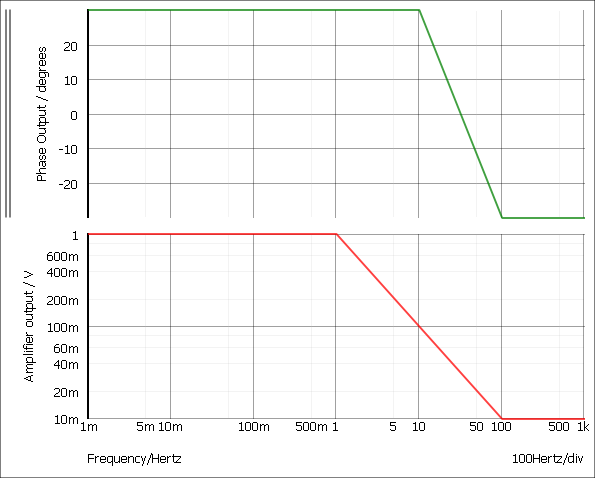
Table_M(0.01,1,30, 1,1,30, 10,0.1,30, 100,0.01,-30)
The above defines a response with a gain of 1 and a phase shift of 30 degrees from 0.01Hz to 1Hz. From 1Hz to 10Hz the gain falls from 1 to 0.1 with the phase shift remaining at 30 degrees. From 10Hz to 100Hz the gain falls from 0.1 to 0.01 and the phase changes from 30 to -30 degrees.
In real life it is not possible to implement a characteristic with the above behaviour as it is non-causal. However, it can be implemented if a suitable delay is added to the characteristic. The delay may be added using the DELAY parameter. Alternatively it may be added to the Laplace expression using ???MATH???exp(-delay.s)???MATH???. E.g:
Table_M(0.01,1,30, 1,1,30, 10,0.1,30, 100,0.01,-30) * exp(-s*2)
The above adds a 2 second delay.
For ease of reading, each triplet in the table may be placed on a separate line by prefixing each line with a '+' character. E.g.
Table_M(
+ 0.01,		1,		30,
+ 1,		1,		30,
+ 10,		0.1,		30,
+ 100,		0.01,		-30)
Interpolation Between defined frequency points, the Laplace transfer function finds the magnitude and phase using interpolation. The interpolation is performed logarithmically on the magnitude data. Values outside the table frequency range are defined by their respective end points.
If the table contains zero frequency terms or zero magnitude terms, the values are replaced with the values of parameters TABLE_ZERO_FREQ and TABLE_ZERO_MAG parameters respectively. This is because the interpolation is performed logarithmically and this requires all values to be > 0.
For the above example the magnitude and phase are shown below:
Parameters
Parameters (defined with .PARAM) may be used in Laplace expressions.
Implementation
The Laplace transfer function is implemented using a convolution method.
In the frequency domain, a linear system may be represented by: \[ Vout(s) = Vin(s).f(s) \] where ???MATH???f(s)???MATH??? is the transfer function.
In the time domain the same system may be represented by: \[ Vout(t) = Vin(t) \ast f(t) \] Where ???MATH???f(t)???MATH??? is the impulse response of ???MATH???f(s)???MATH??? and ???MATH???\ast???MATH??? is the convolution operator.
This method is challenging to implement as simple convolution applied to simulation data in its raw form is an ???MATH???\mathcal{O}(n^2)???MATH??? algorithm. This means that the number of computations required at each step is proportional to the square of the number of steps. In practice this becomes unacceptably slow when there are more than about 10000 time steps.
SIMetrix overcomes this performance limitation by using an FFT based fast convolution method with a computation speed of ???MATH???\mathcal{O}(n\log{}^2n)???MATH???. Although dramatically faster, this algorithm requires data to be presented to it at fixed-interval steps which has the effect of placing an upper frequency limit. The actual upper frequency limit can be arbitrarily increased by increasing the number of steps (the value of ???MATH???n???MATH???) at the expense of speed and the memory consumed. In practice the default settings work well in most applications and give good performance and accuracy.
| Analytical | Matches the Laplace transform to known analytical solutions. For example ???MATH???\frac{1}{\sqrt{}(s)}???MATH??? has the impulse response of ???MATH???\frac{1}{2.\pi\sqrt{t}}???MATH???. SIMetrix will automatically detect this and other known Laplace transforms. |
| Inverse FFT | Calculates the inverse Fourier transform of the Laplace expression. This is a general purpose method that can be applied to a wide-range of Laplace transforms. However, it has the condition that the impulse response must decay to zero during the time interval. |
| Stehfest method | A method to calculate the inverse Laplace transform. Sometimes this method works for slowly decaying transforms that fail with the inverse FFT method. |
Impulse Response
Problems with Impulse Response Extraction
For the convolution method an impulse response of the Laplace transfer function must be extracted. As mentioned above, three methods are attempted. The inverse FFT method and Stehfest methods are approximate in nature and for this reason, the result from each method is tested. If the test fails the impulse response is rejected and another method is attempted. If all methods fail the simulation will abort.
Transfer functions that decay slowly are likely to fail the inverse FFT method as this method requires that the impulse response decay to zero or nearly to zero. If the Stehfest method also fails, the problem can sometimes be resolved by increasing the inverse FFT size. This is controlled by the IMPULSE_IFFT_N parameter. This increases the duration over which the inverse FFT is evaluated so providing a longer time to decay.
In many situations the impulse response extraction fails because the transfer function is non-causal. This means that it has a response in negative time. Non-causal transfer functions can be made causal by adding a delay.
Impulse Response Testing
If the inverse FFT method or Stehfest methods are used to extract the impulse response, the result is tested before allowing it to be used for the simulation.
The Stehfest method is tested by performing a spot frequency check. That is the impulse response is used to measure the gain of a sequence of sine waves in the time domain to check that the magnitudes match to that predicted in the frequency domain. The parameters IMPULSE_TEST_FMAX and IMPULSE_TEST_FMIN determine the range of frequencies used.
The inverse FFT method may be tested by one of two methods determined by the IMPULSE_IFFT_TEST_METHOD parameter. If set to 0, the spot frequency method as described above will be used. If set to 1, the default, the impulse response is tested by measuring its decay to zero. The inverse FFT method is accurate if the response decays to zero and this is used to test the result.
The tolerance required for the test is set by the IMPULSE_TEST_TOL parameter.
Impulse Response Cache
The impulse response is cached to speed up subsequent simulations with the same response. The cache is located here:
C:\Users\<login-name>\AppData\Roaming\SIMetrix Technologies\SIMetrix810\LaplaceCache
where <login-name> is the name used to log in to your system. This can be deleted at any time. The cache is size limited to 250Mbytes by default. This can be changed using the option variable LaplaceCacheSizeMBytes. Type 'Set LaplaceCacheSizeMBytes=nnn' at the command line to set a new value.
The cache may be disabled by setting the IMPULSE_ENABLE_CACHE parameter to 0.
Impulse Response Analytical Extraction
The impulse response analytical extraction attempts to match the transfer function to one of the following patterns. The parameters ???MATH???a???MATH???, ???MATH???b???MATH???, ???MATH???c???MATH??? etc represent constant values.
| Laplace expression | Impulse response |
| ???MATH???a???MATH??? | ???MATH???a.\delta(t)???MATH??? |
| ???MATH???a/(b.s)???MATH??? | ???MATH???a/b???MATH??? |
| ???MATH???a/\sqrt{b.s}???MATH??? | ???MATH???a/\sqrt{2.\pi.b.t}???MATH??? |
| ???MATH???a/(b.s+c)???MATH??? | ???MATH???a/b.e^{-c/b.t}???MATH??? |
| ???MATH???a/\sqrt{b.s+c}???MATH??? | ???MATH???a*e^{-c.t/b}/\sqrt{b.\pi.t}???MATH??? |
| ???MATH???\sqrt{a/(b.s+c)}???MATH??? | ???MATH???\sqrt{a}*e^{-c.t/b}/\sqrt{b.\pi.t}???MATH??? |
| ???MATH???{\displaystyle \frac{a}{b.s^2+c.s+d}}???MATH??? | ???MATH???{\displaystyle \frac{-(e^{-t/2(\sqrt{p^2-4q}+p)}-e^{t/2(\sqrt{p^2-4q}-p)}}{\sqrt{p^2-4q}}}???MATH??? ???MATH???p=c/b???MATH??? and ???MATH???q=d/b???MATH??? |
| ???MATH???a.e^{b.s}???MATH??? | ???MATH???a.\delta(b+t)???MATH??? |
| ???MATH???a/(b.s^c)???MATH??? | ???MATH???{\displaystyle \frac{a.t^{c-1}}{b.\Gamma(c)}}???MATH??? |
| ???MATH???{\displaystyle \frac{a.s^2+b.s+c}{d.s^2+g.s+f}}???MATH??? | ???MATH???{\textstyle [\frac{-(e^{t.arg2}-e^{t.arg3})*(-p.u+2q+u^2-2v)}{2arg1} - \frac{ (u-p)(e^{t.arg2}+e^{t.arg3}) }{2}+\delta(t)]\frac{a}{d}}???MATH??? ???MATH???p = b/a???MATH??? ???MATH???q = c/a???MATH??? ???MATH???u = g/d???MATH??? ???MATH???v = f/d???MATH??? ???MATH???arg1 = \sqrt{u^2-4v}???MATH??? ???MATH???arg2 = -arg1/2-u/2???MATH??? ???MATH???arg3 = arg1/2-u/2???MATH??? |
| ???MATH???{\displaystyle \frac{a.s+b}{c.s^2+d.s+f}}???MATH??? | ???MATH???{\displaystyle \frac{a}{c}.\frac{(2q-u)(arg2 - arg3) + \sqrt{u^2-4v}(arg3 + arg2)}{2\sqrt{u^2-4v}}}???MATH??? ???MATH???q = b/a???MATH??? ???MATH???u = d/c???MATH??? ???MATH???v = f/c???MATH??? ???MATH???arg2 = e^{t.(\sqrt{u^2-4v}/2-u/2)}???MATH??? ???MATH???arg3 = e^{t.(-\sqrt{u^2-4v}/2-u/2)}???MATH??? |
| ???MATH???{\displaystyle \frac{a.s+b}{c.s+d}}???MATH??? | ???MATH???{\displaystyle \frac{e^{-d.t/c}(b.c-a.d)}{c^2}+\frac{a.\delta(t)}{c}}???MATH??? |
| ???MATH???{\displaystyle \frac{\sqrt{a.s+b}}{\sqrt{c.s+d}}} ???MATH??? | ???MATH???(\alpha.(I1(\alpha.t)-I0(\alpha.t)) + \delta(t)).e^{-\beta.t}.Y???MATH??? ???MATH???Y = \sqrt{a/c}???MATH??? ???MATH???\alpha = (d/c-b/a)/2???MATH??? ???MATH???\beta = (d/c+b/a)/2???MATH??? I0 and I1 are Bessel functions |
The analytic matching algorithm will attempt to match partial expressions as well as the whole expression if they are combined by addition, subtraction or multiplication. For example:
???MATH???(1/(s+1))*exp(-s)???MATH???
will be matched to the product of ???MATH???1/(s+1)???MATH??? and ???MATH???exp(-s)???MATH???. Respectively these have impulse responses of ???MATH???e^{-t}???MATH??? and ???MATH???\delta(1+t)???MATH??? and those two impulse responses will be convolved to yield the final result. Note that this only succeeds if all partial expressions can be matched analytically.
To exploit this method, ensure that the expression is entered in a manner that keeps each partial expression distinct. For example, the following would be matched correctly:
???MATH???1/(s+1)*1/(s+2)???MATH???
as this would be seen as the two partial expressions ???MATH???1/(s+1)???MATH??? and ???MATH???1/(s+2)???MATH??? each of which can be resolved analytically. The final result would be obtained by convolving the two impulse responses.
However the following mathematically identical expression would not be matched:
???MATH???1/((s+1)*(s+2))???MATH???
The analysis algorithm does not attempt to decompose denominator products so this will not be recognised analytically. The above would be extracted using inverse FFT which would usually be successful but might not be if the run time is considerably shorter than the time constant.
Run Time Error Control
During the simulation run the time step is controlled using a truncation error method. The tolerances used for this error control are set using the TRUNC_RELTOL and TRUNC_ABSTOL parameters. The truncation error test may be disabled altogether by setting the TRUNC_TEST parameter to zero.
PSpice LAPLACE and FREQ compatibility
SIMetrix is compatible with PSpice Laplace transfer functions at the netlist level entered in one of these forms
Exxx n1 n2 LAPLACE { input_expression } { laplace_expression }
Gxxx n1 n2 LAPLACE { input_expression } { laplace_expression }

Exxx n1 n2 FREQ {input_expression} [keyword1] [keyword2] table_values DELAY=delay
Gxxx n1 n2 FREQ {input_expression} [keyword1] [keyword2] table_values DELAY=delay
| input_expression | Expression to define input signal. E.g. V(vin) |
| laplace_expression | Laplace transfer function |
| keyword1 and keyword2 | RAD, MAG, DB, DEG or R_I |
| table_values | table look up entries in groups of three |
| delay | additional delay |
SIMetrix will implement the PSpice expression in the best way possible. If the Laplace expression can be expressed as a quotient of polynomials, the lumped model (see Laplace Transfer Function - Lumped Implementation) will be used instead of the convolution model as long as it does not contain any parameters.
| ◄ Laplace Transfer Function - Lumped Implementation | Lossy Transmission Line ▶ |