2.0 Transient Analysis Settings
At first glance, the SIMPLIS transient analysis appear to be just like a SPICE transient analysis. Both simulators have start and stop time controls and a way to control the number of data points.
Behind the scenes, the SIMPLIS transient simulation actually bears little resemblance to the SPICE transient simulation. In this topic you will learn how and why the SIMPLIS transient simulation is different from a SPICE transient simulation.
In this topic:
Key Concepts
This topic addresses the following key concepts:
- SIMPLIS thinks of your schematic as sequence of individual, distinct circuits, these are called topologies.
- SIMPLIS saves these topologies for reuse during the simulation, effectively learning the circuit.
- Previous simulation states, called snapshots, can automatically be loaded into the simulator, allowing a simulation to start at a previously known state.
- The number of plot points increases the fidelity of the displayed waveform, but not the numerical accuracy of the SIMPLIS simulation. SIMPLIS always uses the highest numerical accuracy, for every simulation.
What You Will Learn
In this topic, you will learn the following:
- How SIMPLIS saves switching instance data, or topologies, during the simulation.
- What constitutes a new topology.
- How to set basic and advanced transient analysis settings.
- How the Force New Analysis option disables transient snapshot loading.
Getting Started
To get started you will open a schematic and examine the transient analysis settings.
Exercise #1: SIMPLIS Transient Analysis Settings
- Open the schematic titled 2.1_SIMPLIS_tutorial_buck_converter.sxsch from the Module_2_Examples.zip file. This is the same circuit used in section 1, but with a few modifications to the analysis parameters and the initial conditions.
- From the schematic menu, select , or press the F8 key. Result: The Choose SIMPLIS Analysis dialog opens.
- Click on the Transient tab to view the transient analysis settings.
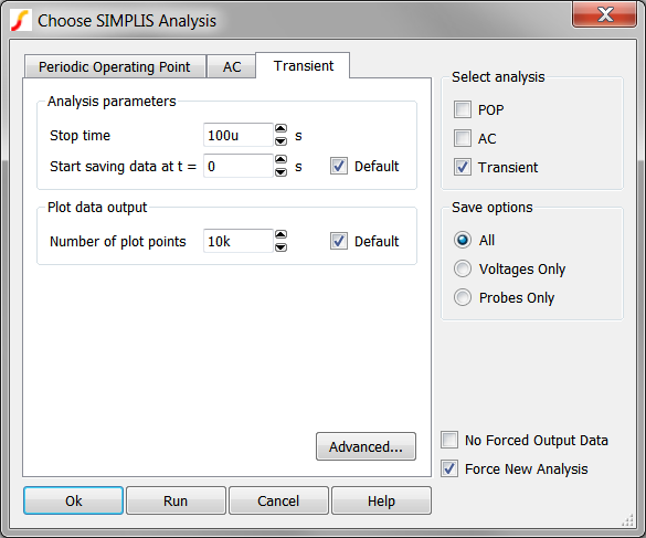
Exercise #1: Discussion
The SIMPLIS Transient analysis settings are divided into two groups:
- Analysis Parameters
- Data Plotting Parameters
There is a distinct difference between the Analysis parameters and the Plot data output parameters. The Analysis parameters, in particular the Stop time, define the time interval which SIMPLIS will collect switching instance data. Switching instance data is the state of each topology as the circuit switches from one PWL topology to the next. The switching instance data is internal to SIMPLIS and is not output to the waveform viewer as vectors.
The Plot data output has only one parameter Number of plot points, which sets the number of additional plot points added to the output waveforms. By increasing the Number of plot points parameter, you increase the fidelity of the waveforms displayed on the waveform viewer, but this doesn't change the accuracy of the simulation.
Exercise #2: Run a Transient Analysis
You will now run the transient simulation from 0 to 100μs. Before launching the simulation, you will clear the messages from the SIMPLIS Status window. To run the simulation,
- Click Cancel on the Choose Analysis dialog.
- Open the SIMPLIS Status Window. The keyboard shortcut Ctrl+Space will bring the window into focus.
- Clear the messages by clicking on the Clear Messages button.
- Move the mouse anywhere in the schematic and click the left mouse button to bring the SIMetrix/SIMPLIS main window into focus.
- Press F9 to run the simulation.Result: While SIMPLIS runs the transient analysis on the circuit, the SIMPLIS Status window outputs the progress of the simulation.The SIMPLIS Status window contains information about the progress of the simuation:
	TIME-DOMAIN TRANSIENT ANALYSIS


                                   New topology #7
                                   New topology #8
                                   New topology #9
                                   New topology #10
                                   New topology #11
                                   New topology #12
                                   New topology #13
                                   New topology #14
                                   New topology #15
                                   New topology #16
01                                 New topology #17
                                   New topology #18
   02                              New topology #19
                                   New topology #20
                                   New topology #21
                                   New topology #22
                                   New topology #23
                                   New topology #24
                                   New topology #25
                                   New topology #26
      03                           New topology #27
         04                        New topology #28
                                   New topology #29
            05                     New topology #30
                                   New topology #31
               06                  New topology #32
                                   New topology #33
                  07 08 09 10
11 12 13 14 15 16 17 18            New topology #34
                                   New topology #35
                                   New topology #36
                        19 20
21 22 23 24 25 26 27 28 29 30
31 32 33 34 35 36 37 38 39 40
41 42 43 44 45 46 47 48 49 50
51 52 53 54 55 56 57 58 59 60
61 62 63 64 65 66 67 68 69 70
71 72 73 74 75 76 77 78 79 80
81 82 83 84 85 86 87 88 89 90
91 92 93 94 95 96 97 98 99 100
                                   Elapsed time   :  0 hr  0 min  1    sec
                                   CPU time       :  0 hr  0 min  0.17 sec
                                   Simulation time: 1.000000000000e-004 sec


Writing pertinent data files ...
Leaving SIMPLIS.
Exercise #2: Discussion
There are primarily two types of messages output to the SIMPLIS Status window during this transient simulation:
- The Percent Complete, shown on the left hand side as a series of two-digit numbers from 01 to 100.
- The New topology information on the right hand side.
These messages are output in sequential order, for example, between 6 and 7% complete, the simulator found New topology #33. New topologies are described next.
New Topologies
During a SIMPLIS simulation, the PWL circuit will transition between multiple unique PWL topologies. For example, in a typical buck converter, there exists an state where the high-side switch is on, and energy is both delivered to the output and stored in the inductor. This is followed by a freewheeling phase where the low-side switch is on, and energy stored in the inductor is delivered to the load. This simple example represents two PWL topologies. As the SIMPLIS simulation progresses, SIMPLIS identifies these topologies and stores the topology information for later use. The first time a unique topology is encountered, SIMPLIS declares this to be a new topology. In plain terms, SIMPLIS learns the circuit as the simulation progresses.
New Topologies vs. Known Topologies
The first time SIMPLIS encounters a particular topology, the topology is declared a new topology, a number of computationally intensive tasks are performed, and the information is stored for future use. This topology is now a known topology and information about the topology is resident in memory for future use. As the simulation progresses through topological changes, SIMPLIS adds new topologies to the memory store, and retrieves known topologies from memory. This machine learning process is one characteristic of SIMPLIS which is different than SPICE.
Since it takes significant computational power to store and retrieve the topology information, the more topologies a circuit transitions through, the slower the SIMPLIS simulation will be.
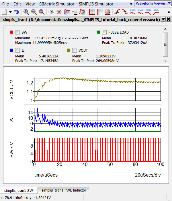
Exercise #2: Conclusions
If you examine both the waveforms and the status window, you will see that the last New topology was found at around 18% completion. This corresponds to time=18μs on the transient analysis graph. After this time, the circuit is settling into a final, steady-state, and SIMPLIS has learned all topologies in this circuit.
Force New Analysis and Snapshots
At this point you know SIMPLIS has the ability to very closely save the state of the circuit for future use. By default SIMPLIS saves the state, or Snapshot, of the PWL circuit at time=0, at the Stop time, and at 10 roughly equally spaced time intervals between the start and stop times. These snapshots are available for use in a future simulation. In the previous exercises, you have told SIMPLIS to ignore any previous state information by checking the Force new analysis check box, this option tells SIMPLIS to not load snapshot information.
Consider the following real-world simulation situation:
You are developing a PFC controller and would like to closely examine the startup behavior of the circuit. Your first task is to examine the first two complete line cycles (40ms at 50Hz Line), then move onto the successive line cycles. Since PFC converters are switching at a high frequency and have a line frequency input which is much lower frequency, these converters are computationally intensive. To save time, it would be nice to be able to store the state after any number of line cycles as a snapshot, and pick up that snapshot in a future simulation. In the next exercise you will load a snapshot for a PFC converter.
Exercise #3: Loading previous simulation states
An exercise will demonstrate loading the snapshot from a previous simulation. To get started,
- Close all open schematics without saving.
- Open the 2.2_PFC_Critical_Conduction_Mode.sxsch example schematic.
- Close the waveform viewer.
- Open the SIMPLIS Status Window. The keyboard shortcut Ctrl+Space will bring the window into focus.
- Clear the messages by clicking on the "Clear Messages" button.
- From the schematic menu, select , or press the F8 key.
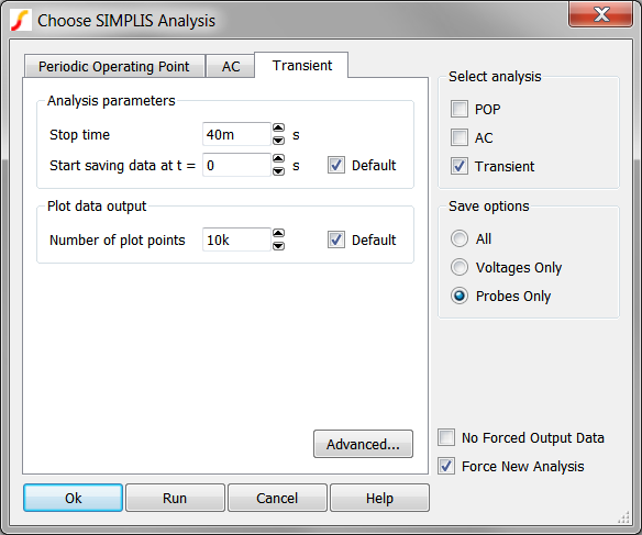 These default analysis settings will ignore previous Snapshot
information, and will simulate from 0 to 40ms.
These default analysis settings will ignore previous Snapshot
information, and will simulate from 0 to 40ms. - Run the simulation.
The simulation will take approximately 15-20 seconds to complete. The waveform viewer will open to display the control signals:
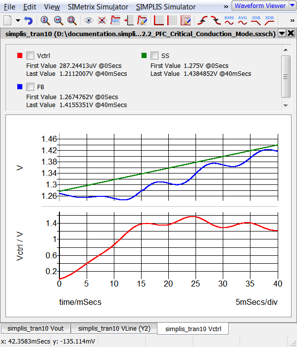
Now you will tell SIMPLIS to load the state of the PFC circuit at 40ms, and continue to simulate for another 60ms to the stop time of 100ms.
- From the schematic menu, select The keyboard shortcut F8 will execute this menu item.
- Make the following changes to the dialog:
- Un-check the Force New Analysis check box.
- Set the Stop time to 100m.
- Set the Start saving data to 40m. The configured dialog should
appear exactly as follows:
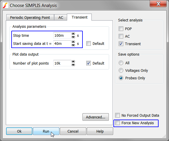
- Double check the dialog appears exactly as above. You will not get a second chance if the analysis settings are incorrect.
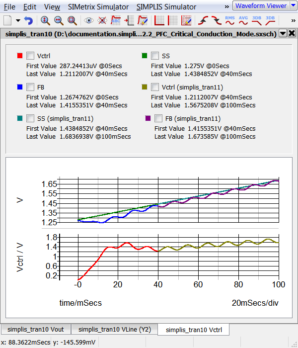
- Run the simulation by clicking on the Run button. Result: SIMPLIS loads the state of the simulation at 40ms, and simulates to 100ms.
The waveform viewer now shows two sets of curves, one each from each simulation run. The second simulation starts where the first simulation left off, at 40ms.
If you look carefully in the SIMPLIS Status window, you will see a message (you may have to scroll up to find the message near the top):
Reading the state/snapshot of the simulation at t = 4.00000000e-002 sec
This message indicates that at the start of the transient analysis, SIMPLIS has loaded the previous Snapshot information at time=40ms.
What can go wrong?
A number of items will prevent SIMPLIS from loading snapshot information:
- There is no previously saved snapshot information to load.
- The Force new analysis check box is checked.
- The circuit has materially changed since the last snapshot was taken.
- No snapshot is available to load because of the analysis parameter settings. This will be explained next.
Advanced Transient Analysis Dialog
Clicking on the Advanced.. button will open the Advanced Transient Options dialog:To save additional snapshots in between the default Snapshot at time=0 and at the Stop time,
- Check the Enable snapshot output check box. Result: The Snapshot interval and Max snapshots controls are enabled.
- Enter the desired snapshot interval in seconds in the Snapshot interval entry.
- Enter the maximum number of snapshots in the Max snapshots entry. Tip: The maximum number of snapshots will over-ride your Snapshot interval if a conflict arises.
Further Study
( not covered in class )
Reading the state/snapshot of the simulation at t = 3.85162005e-002 sec
Conclusions and Key Points to Remember
- SIMPLIS saves switching instance data representing each PWL topology as the simulation progresses.
- SIMPLIS "learns" the circuit during the simulation.
- The new topologies are concentrated toward the beginning of the simulation time window.
- A particular time slice of data can be output with the Start plotting data and Stop plotting data parameters.
- Force new analysis tells SIMPLIS to ignore all previously saved state information.
- Snapshots allow you to save time by restarting a simulation from a previously stored state.