Performance Analysis and Histograms
In this topic:
Overview
When running multi-step analyses which generate multiple curves, it is often useful to be able to plot some characteristic of each curve against the stepped value. For example, suppose you wished to investigate the load response of a power supply circuit and wanted to plot the fall in output voltage vs transient current load. To do this you would set up a transient analysis to repeat a number of times with a varying load current. (See Multi-step Analyses to learn how to do this). After the run is complete you can plot a complete set of curves, take cursor measurements and manually produce a plot of voltage drop vs. load current. This is of course is quite a time consuming and error prone activity.
Fortunately, SIMetrix has a means of automating this procedure. A range of functions - sometimes known as goal functions - are available that perform a computation on a complete curve to create a single value. By applying one or a combination of these functions on the results of a multi-step analysis, a curve of the goal function versus the stepped variable may be created.
This feature is especially useful for Monte Carlo analysis in which case you would most likely wish to plot a histogram.
We start with an example and in fact it is a power supply whose load response we wish to investigate.
Example
The following circuit is a model of a hybrid linear-switching 5V PSU. See Work/Examples/HybridPSU/5vpsu_v1.sxsch
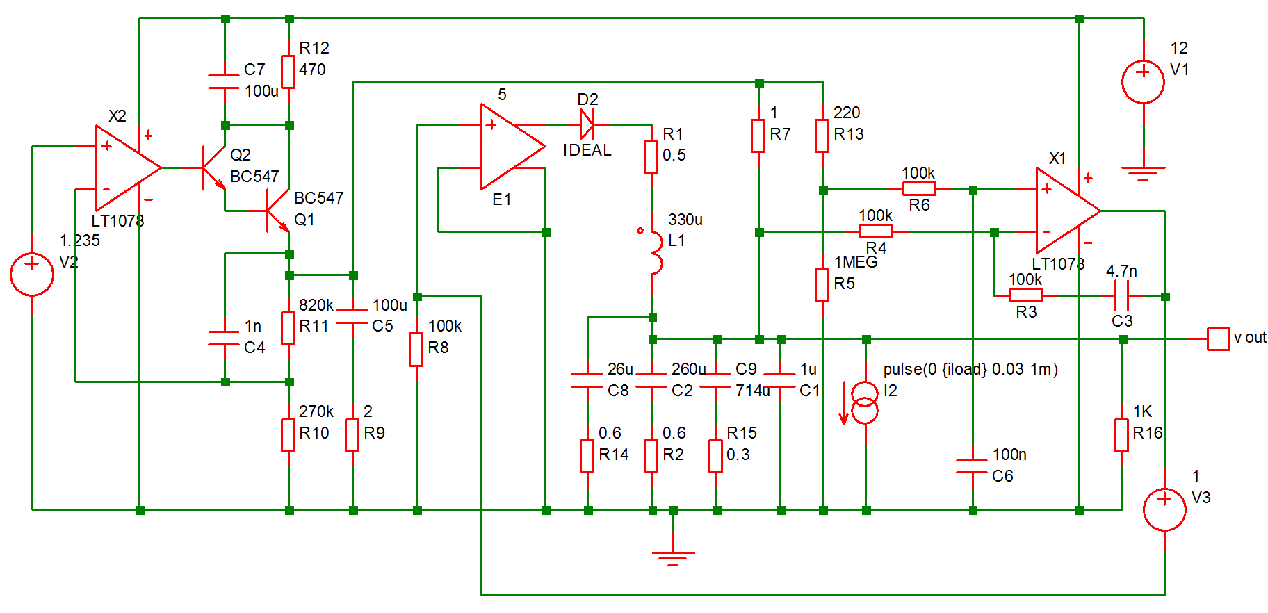
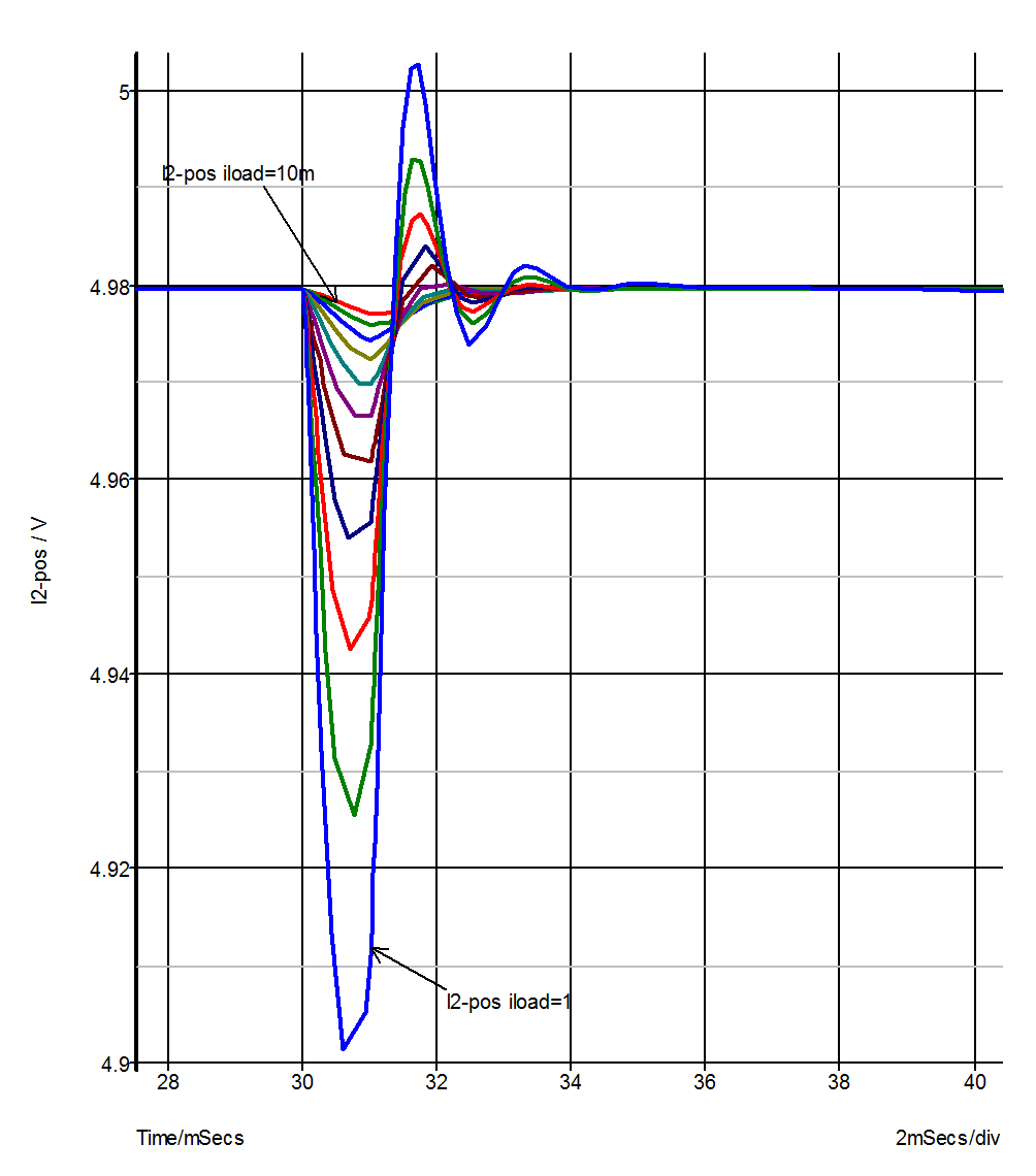
I2 provides a current that is switched on for 1mS after a short delay. A multi-step analysis is set up so that the load current is varied from 10mA to 1A. The output for all runs is:
We will now plot the a graph of the voltage drop vs the load current. This is the procedure:
- Select menu
-
You will see a dialog box very similar to that shown in Plotting an Arbitrary Expression. In the expression box you must enter an expression that resolves to a single value for each curve. For this example we use:
yatx(vout, 0) - minimum(vout)
yatx(vout, 0) returns the value of vout when time=0. minimum(vout) returns the minimum value found on the curve. The end result is the drop in voltage when the load pulse occurs. Click Ok and the following curve should appear: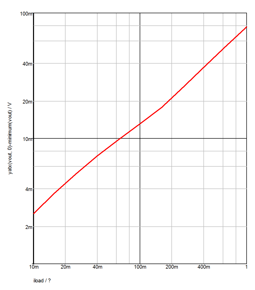
Histograms
The procedure for histograms is the same except that you should use the menu instead. Here is another example.
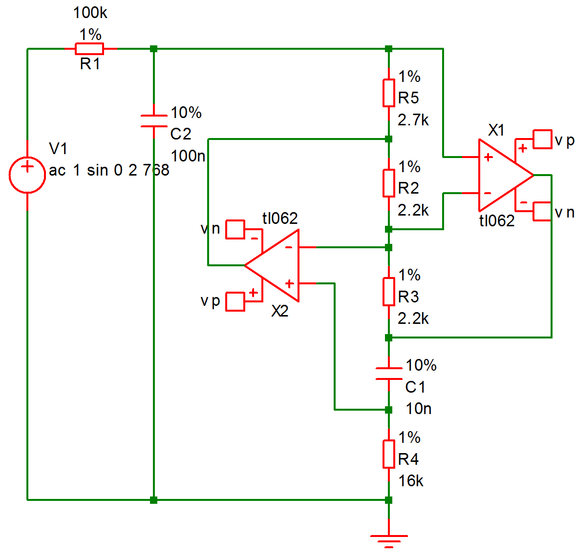
This is a design for an active band-pass filter using the simulated inductor method. See Examples/MonteCarlo/768Hz_bandpass.sxsch. We want to plot a histogram of the centre frequency of the filter.
The example circuit has been set up to do 100 runs. This won't take long to run, less than 10 seconds on most machines. This is the procedure:
- Run the simulation using F9 or equivalent menu.
- Select menu
- Left click on the output of the filter. This is the junction of R1 and C2.
-
You should see R1_P appear in the expression box. We must now modify this with a goal function that returns the centre frequency. The function CentreFreq will do this. This measures the centre frequency by calculating the half way point between the intersections at some specified value below the peak. Typically you would use 3dB.
Modify the value in the expression box so that it reads:
CentreFreq(R1_p, 3)
- At this stage you can optionally modify the graph setting to enter your own axis labels etc. Now close the box. This is what you should see:
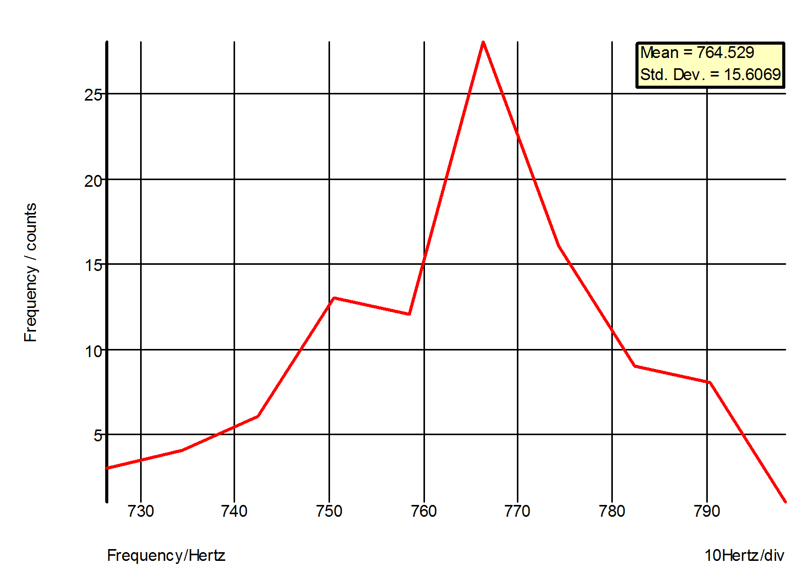 Note that the mean and standard deviation are automatically calculated.
Histograms for Single Step Monte Carlo Sweeps
An example of this type of run is shown in the sectionMonte Carlo. These runs produce only a single curve with each point in the curve the result of the Monte Carlo analysis. With these runs you do not need to apply a goal function, just enter the name of the signal you wish to analyse. To illustrate this we will use the same example as shown in the sectionMonte Carlo.
- Open the example circuit Examples/Sweep/AC_Param_Monte
- Run simulation.
- Select menu
-
Left click on '+' pin of the differential amplifier E1. You should see R4_N appear in the box. Now enter a '-' after this then click on the '-' pin of the E1. This is what should be in the box:
R4_N-R3_N
- Close box. You should see something like this:
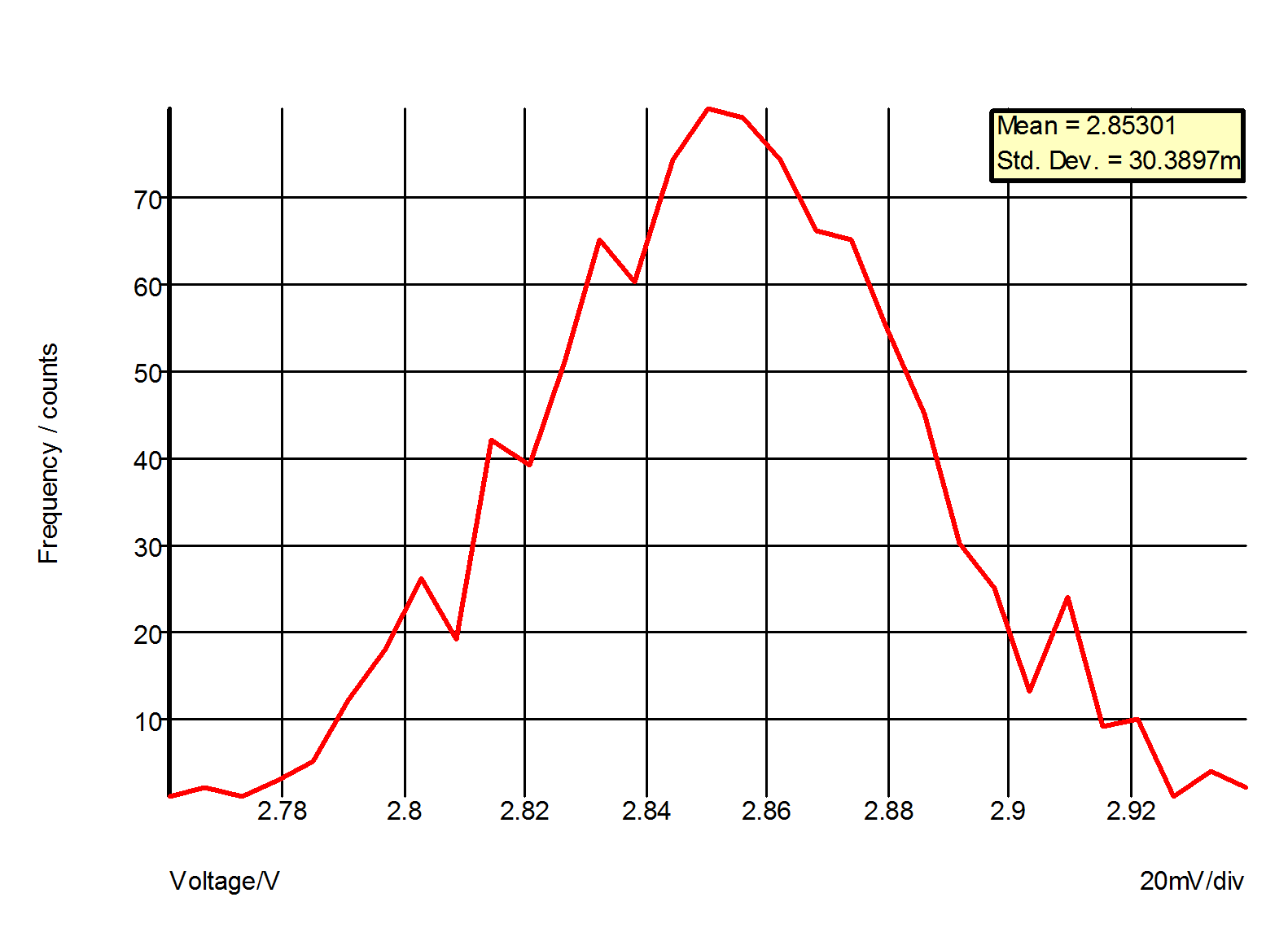 This is a histogram showing the distribution of the gain of the amplifier at 100kHz.
Goal Functions
A range of functions are available to process curve data. Some of these are primitive and others use the user defined function mechanism. Primitive functions are compiled into the binary executable file while user defined functions are defined as scripts and are installed at functions at start up. User defined functions can be modified and you may also define your own. For more information refer to Script Reference Manual/Applications/User Defined Script Based Functions.
The functions described here aren't the only functions that may be used in the expression for performance analysis. They are simply the ones that can convert the array data that the simulator generates into a single value with some useful meaning. There are many other functions that process simulation vectors to produce another vector for example: log; sqrt; sin; cos and many more. These are defined in Script Reference Manual/Function Reference.
Of particular interest is the Truncate function. This selects data over a given X range so you can apply a goal function to work on only a specific part of the data.
Primitive Functions
The following primitive functions may be used as goal functions. Not all actually return a single value. Some return an array and the result would need to be indexed. Maxima is an example.
| Name | Description |
| Maxima(real [, real, string]) | Returns array of all maximum turning points |
| Maximum(real/complex [, real, real]) | Returns the largest value in a given range. |
| Mean(real/complex) | Returns the mean of all values. (You should not use this for transient analysis data as it fails to take account of the varying step size. Use Mean1 instead.) |
| Mean1(real [, real, real]) | Finds the true mean accounting for the interval between data points |
| Minima(real [, real, string]) | Returns array of all minimum turning points. |
| Minimum(real/complex) | Returns the largest value in a given range. |
| RMS1(real [, real, real]) | Finds RMS value of data |
| SumNoise(real [, real, real]) | Integrates noise data to find total noise in the specified range. |
| XFromY(real, real [, real, real]) | Returns an array of X values at a given Y value. |
| YFromX(real, real [, real]) | Returns an array of Y values at a given X value. |
User Defined Functions
The following functions are defined using the user defined functions mechanism. They are defined as scripts but behave like functions.
| Name | Description |
| BPBW(data, db_down) | Band-pass bandwidth. |
| Bandwidth(data, db_down) | Same as BPBW |
| CentreFreq(data, db_down) | Centre frequency |
| Duty(data, [threshold]) | Duty cycle of first pulse |
| Fall(data, [start, end]) | Fall time |
| Frequency(data, [threshold]) | Average frequency |
| GainMargin(data, phaseInstabilityPoint) | Gain Margin |
| HPBW(data, db_down) | High pass bandwidth |
| LPBW(data, db_down) | Low pass bandwidth |
| Overshoot(data, [start, end]) | Overshoot |
| PeakToPeak(data, [start, end]) | Peak to Peak |
| Period(data, [threshold]) | Period of first cycle. |
| PhaseMargin(data, phaseInstabilityPoint) | Phase Margin |
| PulseWidth(data, [threshold]) | Pulse width of first cycle |
| Rise(data, [start, end]) | Rise time |
| XatNthY(data, yValue, n) | X value at the Nth Y crossing |
| XatNthYn(data, yValue, n) | X value at the Nth Y crossing with negative slope |
| XatNthYp(data, yValue, n) | X value at the Nth Y crossing with positive slope |
| XatNthYpct(data, yValue, n) | X value at the Nth Y crossing. y value specified as a percentage. |
| YatX(data, xValue) | Y value at xValue |
| YatXpct(data, xValue) | Y value at xValue specified as a percentage |
BPBW, Bandwidth
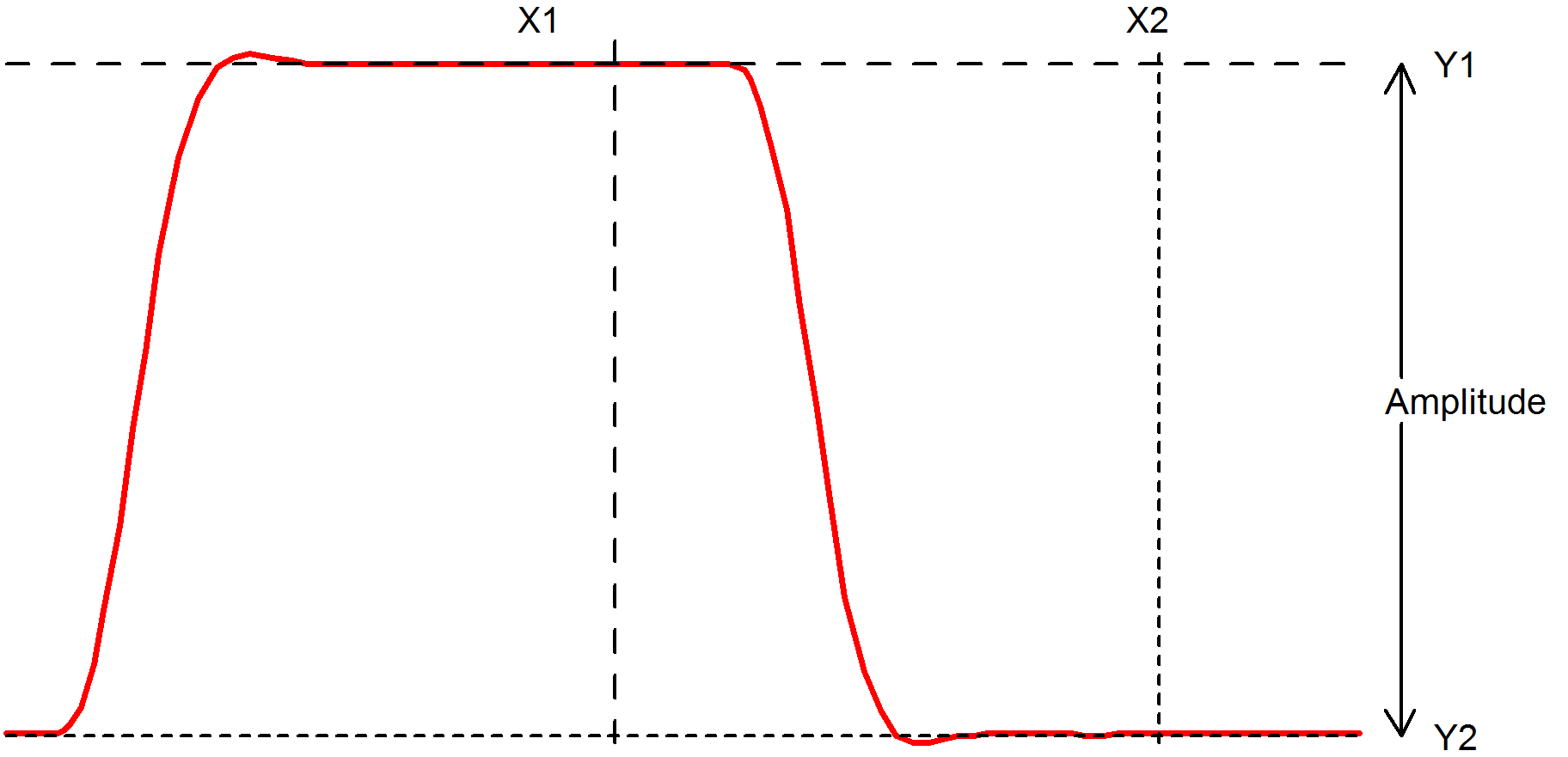
BPBW(data, db_down)Finds the bandwidth of a band pass response. This is illustrated by the following graph
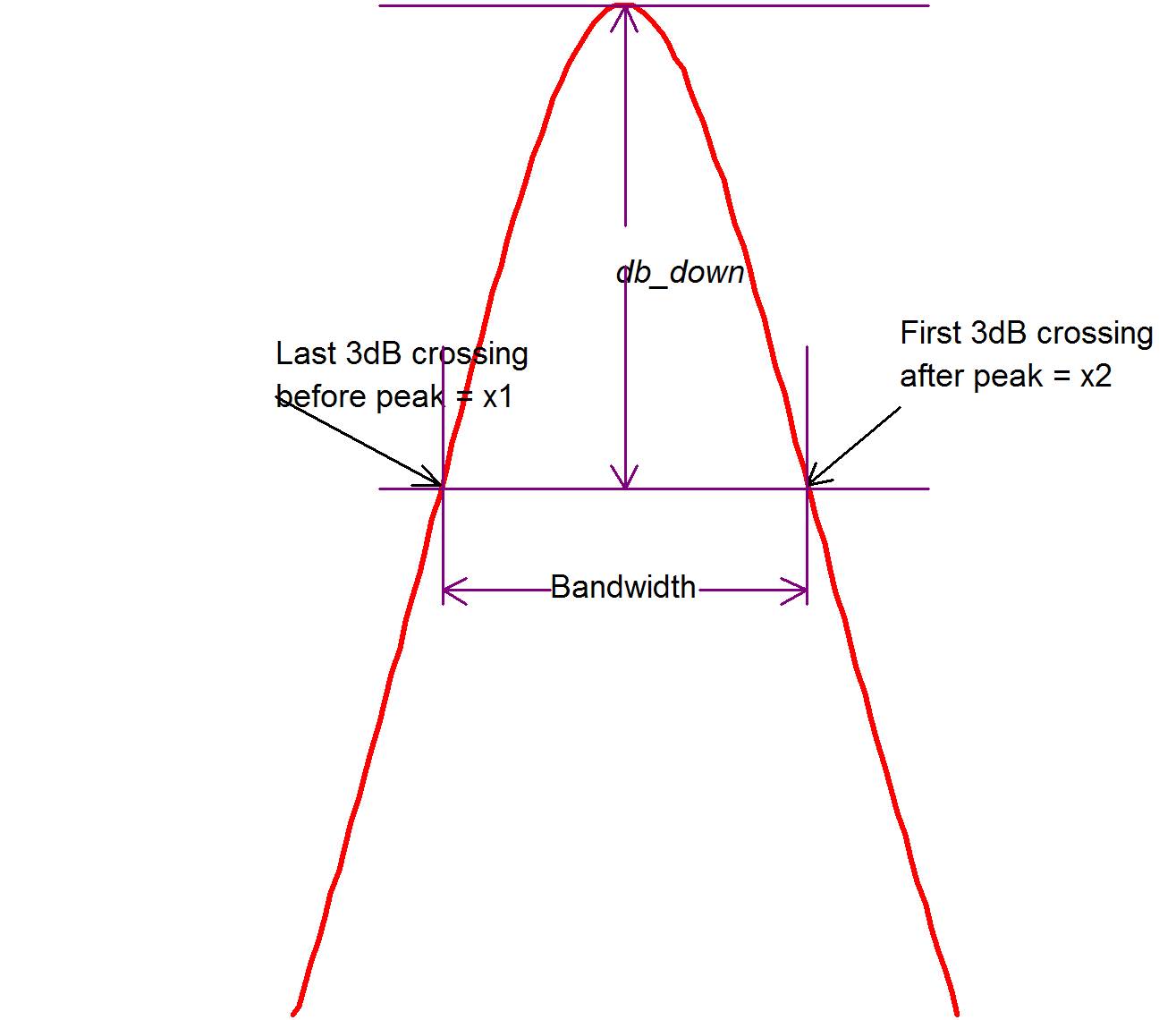
Function return x2-x1 as shown in the above diagram.
Note that data is assumed to be raw simulation data and may be complex. It must not be in dBs.
Implemented by built-in script uf_bandwidth. Source may be obtained from the install CD (see ).
CentreFreq, CenterFreq
CentreFreq(data, db_down)
See diagram in BPBW, Bandwidth. Function returns ???MATH???(x1+x2)/2???MATH???.
Both British and North American spellings of centre (center) are accepted.
Implemented by built-in script uf_centre_freq. Source may be obtained from the install CD (see Install CD).
Duty
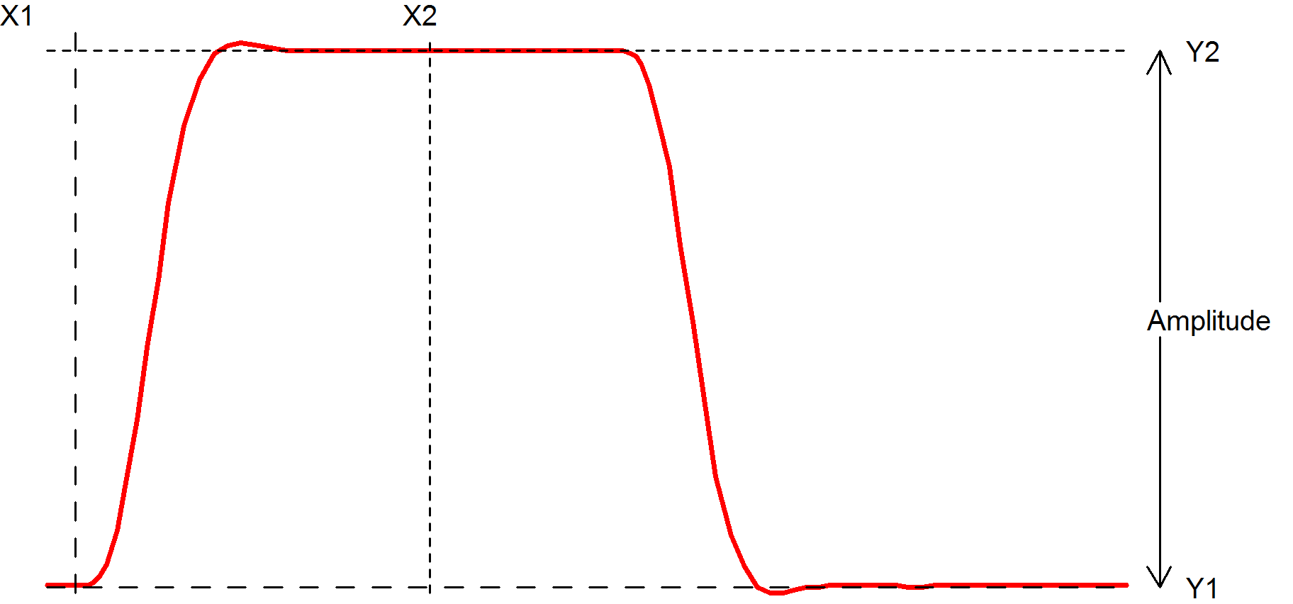
Duty(data, [threshold])
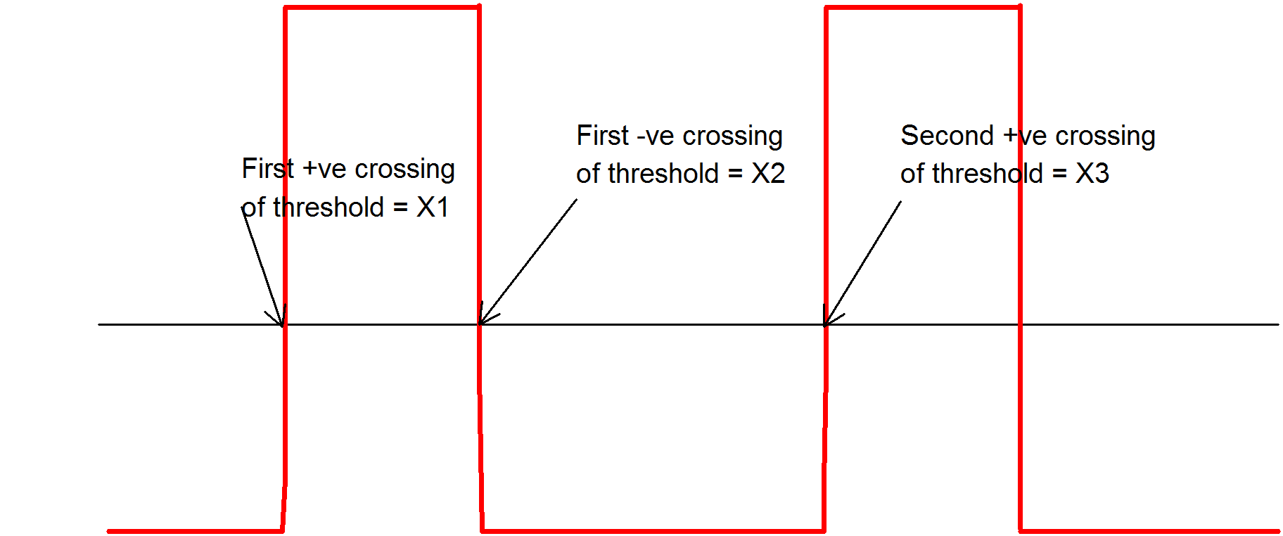
Function returns (X2-X1)/(X3-X1), where X1, X2 and X3 are defined in the above graph.
Default value for threshold is
(Ymax+Ymin)/2
Where Ymax = largest value in data and Ymin in smallest value in data.
Implemented by built-in script uf_duty. Source may be obtained from the install CD (see Install CD).
Fall
Fall(data, [xStart, xEnd])
Function returns the 10% to 90% fall time of the first falling edge that occurs between x1 and x2. The 10% point is at y threshold Y1 + (Y2-Y1)*0.1 and the 90% point is at y threshold Y1 + (Y2-Y1)*0.9.
- If xStart is specified, X1=xStart otherwise X1 = x value of first point in data.
- If xEnd is specified, X2=xEnd otherwise X2 = x value of last point in data.
- If xStart is specified, Y1=y value at xStart otherwise Y1 = maximum y value in data.
- If xEnd is specified, Y2=y value at xEnd otherwise Y2 = minimum y value in data.
Implemented by built-in script uf_fall. Source may be obtained from the install CD (see Install CD).
Frequency
Frequency(data, [threshold])
Finds the average frequency of data.
Returns:
\[ (n-1)/(x_n-x_1) \]
- ???MATH???n???MATH??? = the number of positive crossings of threshold
- ???MATH???x_n???MATH??? = the x value of the nth positive crossing of threshold
- ???MATH???x_1???MATH??? = the x value of the first positive crossing of threshold
If threshold is not specified a default value of (ymax+ymin)/2 is used where ymax is the largest value in data and ymin is the smallest value.
Implemented by built-in script uf_frequency. Source may be obtained from the install CD (see Install CD).
GainMargin
GainMargin(data, [phaseInstabilityPoint])
Finds the gain margin in dB of data where data is the complex open loop transfer function of a closed loop system. The gain margin is defined as the factor by which the open loop gain of a system must increase in order to become unstable. phaseInstabilityPoint is the phase at which the system becomes unstable. This is used to allow support for inverting and non-inverting systems. If data represents an inverting system, phaseInstabilityPoint should be zero. If data represents a non-inverting system, phaseInstabilityPoint should be -180.
The function detects the frequencies at which the phase of the system is equal to phaseInstabilityPoint. It then calculates the gain at those frequencies and returns the value that is numerically the smallest. This might be negative indicating that the system is probably already unstable (but could be conditionally stable).
If the phase of the system does not cross the phaseInstabilityPoint then no gain margin can be evaluated and the function will return an empty vector.
HPBW
HPBW(data, db_down)Finds high pass bandwidth.
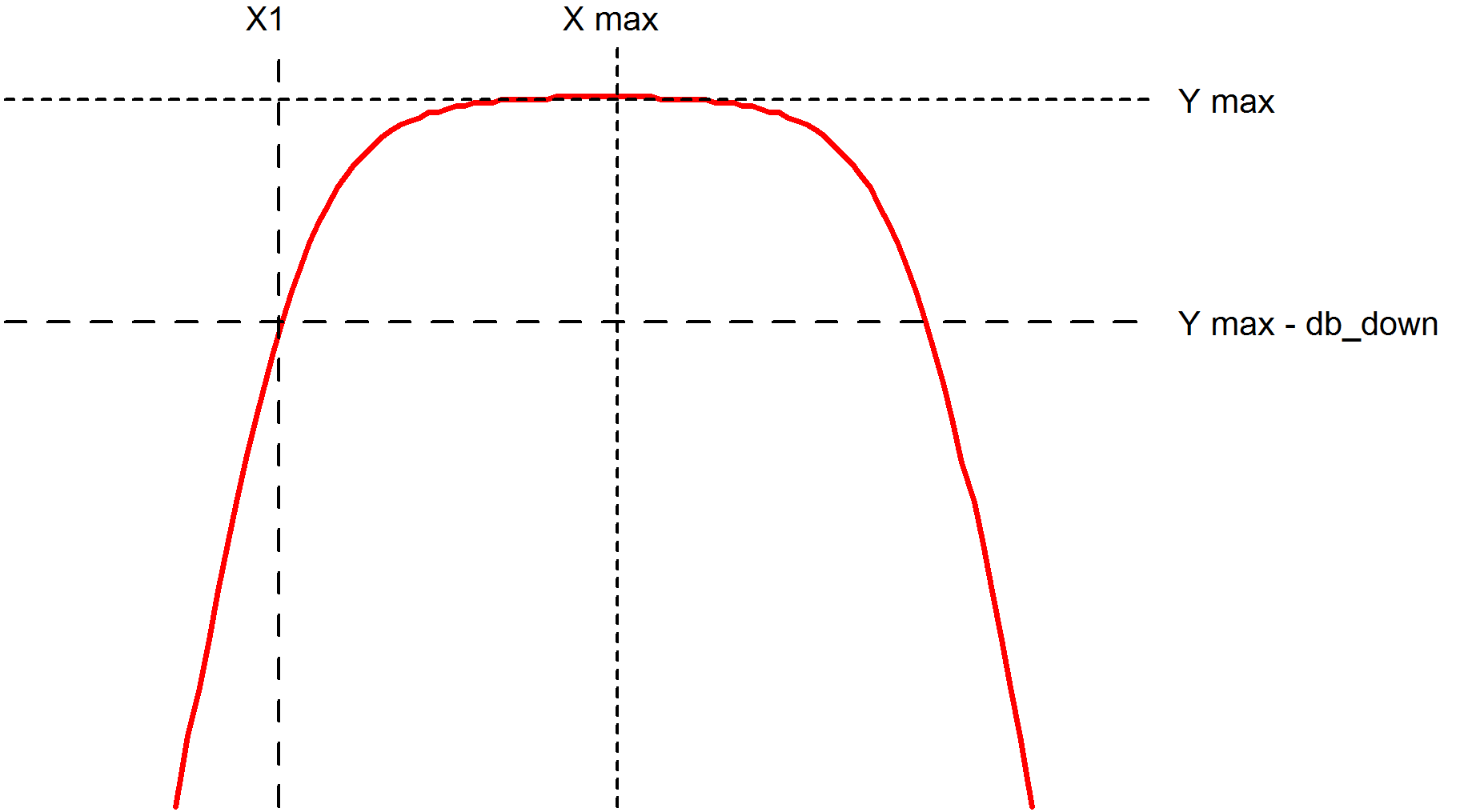
Returns the value of X1 as shown in the above diagram.
- Y max is the y value at the maximum point.
- X max is the x value at the maximum point.
- X1 is the x value of the first point on the curve that crosses (Y max - db_down) starting at X max and scanning right to left.
Note that data is assumed to be raw simulation data and may be complex. It must not be in dBs.
Implemented by built-in script uf_hpbw. Source may be obtained from the install CD (see ).
LPBW
LPBW(data, db_down)Finds low pass bandwidth
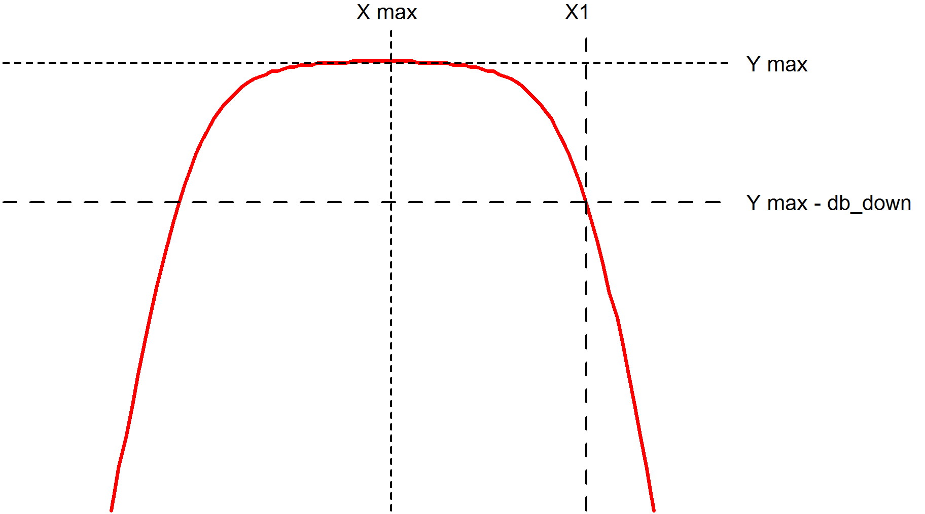
- Y max is the y value at the maximum point.
- X max is the x value at the maximum point.
- X1 is the x value of the first point on the curve that crosses (Y max - db_down) starting at X max and scanning left to right.
Implemented by built-in script uf_lpbw. Source may be obtained from the install CD (see Install CD).
Overshoot
Overshoot(data, [xStart, xEnd])
Finds overshoot in percent.
Returns:
(yMax-yStart)/(yStart-yEnd)
Where
- yMax is the largest value found in the interval between xStart and xEnd.
- yStart is the y value at xStart.
- yEnd is the y value at xEnd.
- If xStart is omitted it defaults to the x value of the first data point.
- If xEnd is omitted it defaults to the x value of the last data point.
Implemented by built-in script uf_overshoot. Source may be obtained from the install CD (see Install CD).
PeakToPeak
PeakToPeak(data, [xStart, xEnd])Returns the difference between the maximum and minimum values found in the data within the interval xStart to xEnd.
- If xStart is omitted it defaults to the x value of the first data point.
- If xEnd is omitted it defaults to the x value of the last data point.
Implemented by built-in script uf_peak_to_peak. Source may be obtained from the install CD (see Install CD).
Period
Period(data, [threshold])Returns the period of the data.
Refer to diagram for the Duty function. The Period function returns:
X3 - X1
Default value for threshold is
(Ymax+Ymin)/2
Where Ymax = largest value in data and Ymin in smallest value in data.
Implemented by built-in script uf_period. Source may be obtained from the install CD (see Install CD).
PhaseMargin
PhaseMargin(data, [phaseInstabilityPoint])Finds the phase margin in dB of data, where data is the complex open loop transfer function of a closed loop system. The phase margin is defined as the angle by which the open loop phase shift of a system must increase in order to become unstable. phaseInstabilityPoint is the phase at which the system becomes unstable. This is used to allow support for inverting and non-inverting systems. If data represents an inverting system, phaseInstabilityPoint should be zero. If data represents a non-inverting system, phaseInstabilityPoint should be -180.
The function detects the frequencies at which the magnitude of the gain is unity. It then calculates the phase shift at those frequencies and returns the value that is numerically the smallest. This might be negative indicating that the system is probably already unstable (but could be conditionally stable).
If the gain of the system does not cross unity then no phase margin can be evaluated and the function will return an empty vector.
PulseWidth
PulseWidth(data, [threshold])Returns the pulse width of the first pulse in the data.
Refer to diagram for the Duty function. The PulseWidth function returns:
X2 - X1
Default value for threshold is
(Ymax+Ymin)/2
Where Ymax = largest value in data and Ymin in smallest value in data.
Implemented by built-in script uf_pulse_width. Source may be obtained from the install CD (see Install CD).
Rise
Rise(data, [xStart, xEnd])
Function returns the 10% to 90% rise time of the first rising edge that occurs between x1 and x2. The 10% point is at y threshold Y1 + (Y2-Y1)*0.1 and the 90% point is at y threshold Y1 + (Y2-Y1)*0.9.
- If xStart is specified, X1=xStart otherwise X1 = x value of first point in data.
- If xEnd is specified, X2=xEnd otherwise X2 = x value of last point in data.
- If xStart is specified, Y1=y value at xStart otherwise Y1 = maximum y value in data.
- If xEnd is specified, Y2=y value at xEnd otherwise Y2 = minimum y value in data.
XatNthY
XatNthY(data, yValue, n)Returns the x value of the data where it crosses yValue for the nth time.
XatNthYn
XatNthYn(data, yValue, n)Returns the x value of the data where it crosses yValue for the nth time with a negative slope.
XatNthYp
XatNthYp(data, yValue, n)Returns the x value of the data where it crosses yValue for the nth time with a positive slope.
XatNthYpct
XatNthYpct(data, yValue, n)As XatNthY but with yValue specified as a percentage of the maximum and minimum values found in the data.
YatX
YatX(data, xValue)Returns the y value of the data at x value = xValue.
YatXpct
YatXpct(data, xValue)As YatX but with xValue specified as a percentage of the total x interval of the data.
| ◄ Viewing DC Operating Point Results | Command Line ▶ |