3.2 SIMPLIS Monte Carlo Analysis
The SIMPLIS Monte Carlo analysis allows you to delve further into a design and see how the design responds to statistical parameter variation. Parameters can also be matched, where two parameter values will track each other every simulation run. Finally, the Monte Carlo log file outputs the actual parameter values used in the simulation and the seed value so that simulation can be repeated.
To download the examples for Module 3, click Module_3_Examples.zip
In this topic:
Key Concepts
This topic addresses the following key concepts:
- Parameter values can be varied using the statistical distribution functions Gauss(), GaussTrunc(), Unif(), and Wc().
- Parameter values can be matched.
- As with the SIMPLIS Mutli-Step Analysis, SIMPLIS can use multiple processor cores to speed up a Monte Carlo simulation.
- You can generate histograms for any scalar measurement, such as the average value of the output voltage, the peak current in a MOSFET, etc.
What You Will Learn
In this topic, you will learn the following:
- How to setup a SIMPLIS Monte Carlo Analysis.
- How to apply the Gauss(), Unif(), and Wc() probability distribution functions to vary parameter values.
- How to match the percentage variation of two or more parameter values.
- How multiple processor cores can be used to reduce the time required to execute a Monte Carlo simulation.
- How to plot histograms.
- How Monte Carlo Seeds are generated.
- How to find the seed number for a simulation and how you can repeat a simulation with a known seed number.
Getting Started
- Open the schematic 3.1_SelfOscillatingConverter_POP.sxsch.
- From the schematic menu, select .Result: The Define SIMPLIS Monte Carlo Analysis dialog opens, displaying the Monte Carlo analysis parameters.
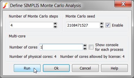
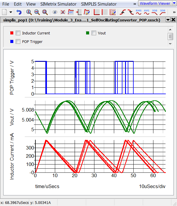
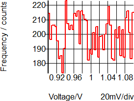
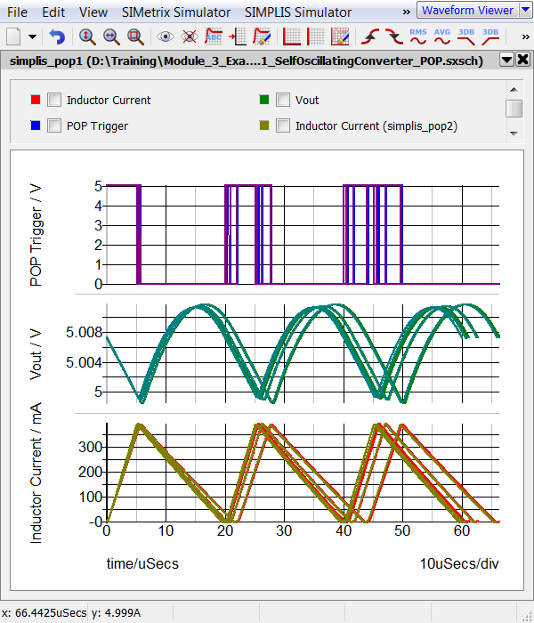
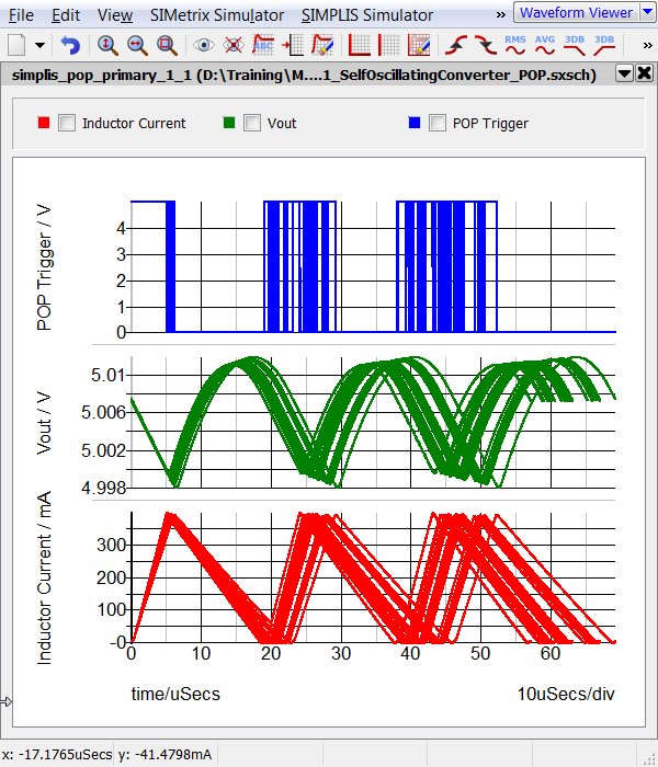
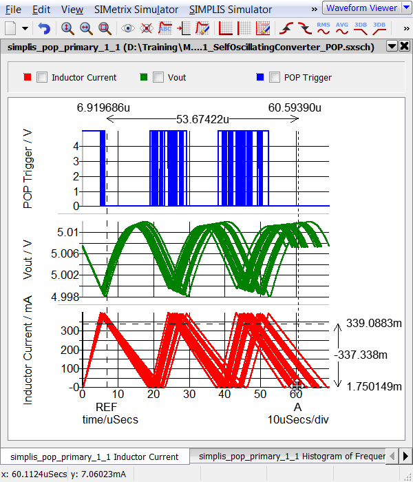
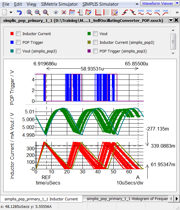
- Click Run.Result: The SIMPLIS Monte Carlo Analysis executes and the waveform viewer opens with the curves from the 4 Monte Carlo steps:
Discussion
The SIMPLIS Monte Carlo Analysis is similar to the SIMPLIS Mutli-Step Analysis except instead of stepping a parameter, the Monte Carlo seed value is stepped. The seed value is used to determine the values of each statistical distribution function used in the design. If no statistical distribution functions are used in the circuit, each seed value will produce the same simulation results.
Statistical Distribution Functions
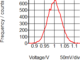
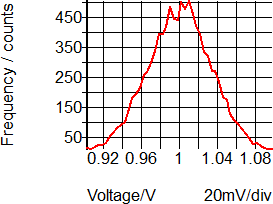
There are three statistical distribution functions for use in the SIMPLIS Monte Carlo Analysis, Gauss(), GaussTrunc(), Unif(), and Wc(). Each of these functions has a different numerical return value when the function is called. The table and histograms pictured below describe each function. The histograms were generated with tol=0.1, or 10%, a mean value of 1, with 10,000 steps (runs), and 50 histogram bins.
| Function | Meaning | Histogram |
| Gauss(tol) |
Gaussian. Returns a random with a mean of 1.0 and a standard deviation of tol/3. Random values have a Gaussian or Normal distribution. Important: The Gauss() function can return values greater than
(1 + tol) and less than (1 - tol). This becomes particularly important
when you are using a large tolerance, as the return value may be outside
of a reasonable range. To use a truncated Gaussian distribution, see
GaussTrunc() below.
|
|
| GaussTrunc(tol) |
Truncated Gaussian. As with Gauss() but values greater than (1 + tol) and less than (1 - tol) are rejected, and the program picks another random number inside the Gaussian distribution. |
|
| Unif(tol) | Uniform. Returns a random value in the range 1.0 +/- tol with a uniform distribution. |
|
| WC(tol) | Worst-Case. Returns either 1.0-tol or 1.0+tol chosen at random. |
|
Assigning Statistical Distribution Functions to Component Values
You assign statistical distribution functions to component values like any other parametrized value. The statistical distribution function and the nominal value must be enclosed in the curly braces {}, indicating the value is an expression to be evaluated. For example, a 1k Ω, 5% resistor with a Gaussian distribution was a value of:
{1k*Gauss(0.05)}
Every Monte Carlo step, the Gauss(0.05) function will return a value with a Gaussian distribution, which is then multiplied by the nominal value and the resistor is assigned this numerical result. On voltage sources and a few other dialogs, you must use the literal property editing dialog to enter text values enclosed in curly braces. In the next exercise you will edit the value of the input voltage source, V1 using the literal property editing method.
Exercise #1: Assign Uniform Distribution to the Input Source V1
- Select the input voltage source V1.Result: The symbol changes from red to blue indicating the symbol is selected.
- Use the keyboard shortcut Shift+F7 to open the literal value editing
dialog.Result: The literal value editing dialog opens:
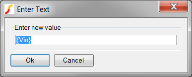
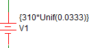
- Enter the uniform distribution: {310*Unif(0.0333)}Result: The configured dialog should appear as follows:
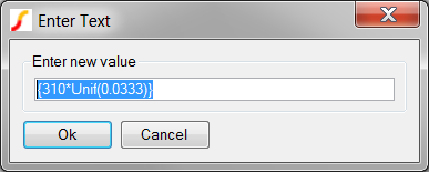
- Click Ok.Result: The property value for the input voltage changes to the uniform distribution of 310V +/- 3.33%.
- From the schematic menu, select Result: The SIMPLIS Monte Carlo Analysis executes and the waveform viewer opens with the curves from the original 4 steps with a constant Input voltage, and the additional 4 steps from the second Monte Carlo Analysis with input voltage variation.
Assigning Matched Statistical Distributions to Component Values
There are times when you may want to have multiple component values which match or track each other. In the SIMPLIS Monte Carlo analysis, this is accomplished by first assigning a variable statement to depend on a statistical distribution function, then using that variable to parametrize the individual matching components. This "master" variable is evaluated once - from then on, the value is constant.
One place where this comes in useful is for PWL inductors, such as L4 in this example circuit. This inductor is used to model the magnetizing inductance of the transformer including saturation effects. In the next exercise you will verify that the inductance of each segment of the inductor L4 is varied in proportion to a Gaussian distribution function.
Exercise #2: Verify L4 Values
- Double click on L4.Result: The Define PWL Inductor: L4 dialog opens:
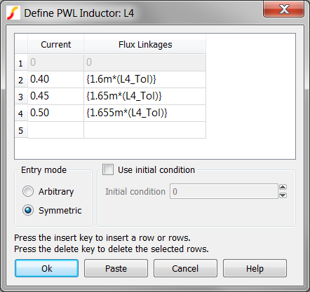
- Note that each Flux Linkage value is multiplied by a constant value L4_Tol. Since the Flux Linkage values are the "y-axis" values, and the slope of each PWL segment represents the inductance of that segment, every PWL segment changes inductance by the same percentage.
- Click Cancel on the Define PWL Inductor: L4 dialog.
- Press F11 to open the command (F11) window. Scroll down to where the
L4_Tol is defined:
.var L4_Tol={Gauss(0.20)}
{ '*' }
{ '*' } L4's tolerance : {L4_Tol}
{ '*' }
The first line assigns the return value of the Gauss(0.20) function to the variable L4_Tol, which is in turn, used to parametrize each y-axis point for L4. The other three lines were purposely placed in the F11 window to allow us to easily see the value returned by the Gauss(0.20) function. Each line is a comment, with the middle line also displaying the value of L4_Tol. - As you did in section 3.0.2 What Actual
Device is Simulated in SIMPLIS?, you look in the deck file to ascertain
exactly what values are used for L4_Tol, and the PWL inductor L4.
From the menu bar, select . Result: the SIMPLIS Deck file opens in the netlist editor.
- To search for the L4 tolerance comment line:
- Use the shortcut key Ctrl+F to open the search dialog.
- Type L4's
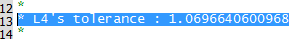
- Click on the Find Next button. Result: The deck file scrolls to line # 13 where the debug comment is located:
- Finally, to search for the actual L4 device instantiation line:
- Use the shortcut key Ctrl+F to open the search dialog.
- Type !L$L4
- Click on the Find Next button three times. Result: The deck file scrolls to line # 49 where the L4 instantiation and its .MODEL line are located:

Piecewise Linear Inductors, such as L4 in this example, are implemented with a .MODEL statement, which in this case, starts on line #50. The PWL points are listed as X,Y pairs starting at X0 and Y0. Notice the X values have the same numerical values you saw in the dialog. The Y-values are all multiplied by the constant value L4_Tol. The L4_Tol is constant because the value is evaluated once per Monte Carlo run, and from that point onwards, the same constant value is used in the expressions for L4_Tol. The value of L4_Tol will almost certainly be different for the next Monte Carlo simulation step.
The value of the L4_Tol variable is 1.0696640600968, which represents a 6.97% increase in inductance values. Calculating the change in inductance is left as an independent study exercise.
SIMPLIS Multi-Core Capability
As with the SIMPLIS_Multi Step Analysis the SIMetrix/SIMPLIS Pro and Elite licenses can use multiple processor cores to simulate the Monte Carlo steps in parallel. Using multiple cores allows multiple step values to be simultaneously simulated, and the simulation time to be reduced. The number of cores allowed by the licenses are:
| License | Number of Physical Cores |
| Pro | 4 |
| Elite | 16 |
In addition to the maximum number of cores allowed by your license, you are obviously limited by the number of cores your computer has. For this limitation, SIMetrix/SIMPLIS only uses the physical cores, not the hyper-threaded cores. In the next exercise you will run a multi-core, multi-step simulation.
Exercise #3: Enable Multi-Core
This exercise assumes your computer has more than one physical core and that you are using a SIMetrix/SIMPLIS Pro license.
- Close the waveform viewer.
- From the schematic menu, select Result: The Define SIMPLIS Monte Carlo Analysis dialog opens with the Monte Carlo configuration information.
- Change the Number of cores to 4, the maximum allowed by the Pro license.
Note: Note: if your machine has either a single core or two cores, the dialog will limit your Number of cores entry. If you have a single core, you can skip this exercise.
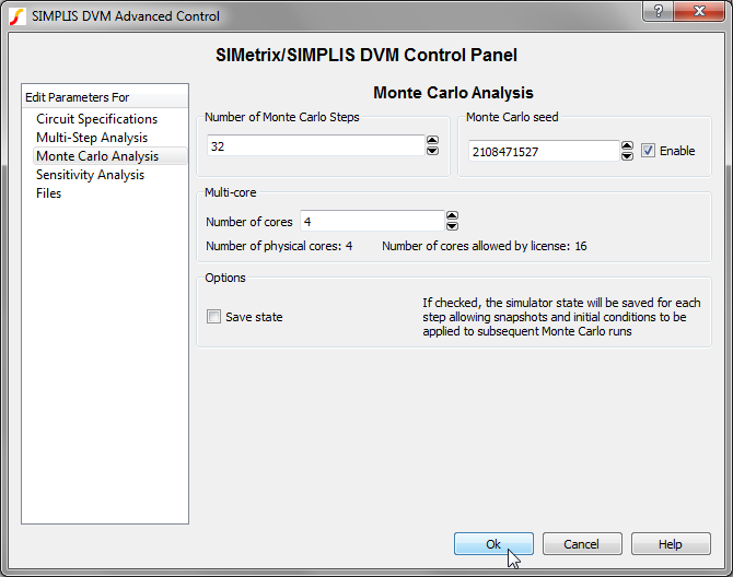
- Change the Number of steps to 32.Result: The configured dialog will appear as follows:
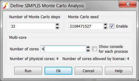
- Click Run.Result: The Monte Carlo simulation runs 32 steps on the maximum number of physical cores.
Plotting Histograms
SIMetrix/SIMPLIS has an extremely powerful histogram plotting function. In the last exercise, you executed 32 simulations to get a valid statistical sample, and the histogram plotting functions requires a minimum of 16 runs. In the next two exercises you will plot the histogram for the converter switching frequency.
Exercise #4: Plotting Histograms
Plotting histograms is different from plotting time domain curves because the histogram function is expecting a single measured value per Monte Carlo step. Compare this to plotting the converter output voltage after a transient simulation - there may be 10,000 points in the output voltage vector, each one representing the voltage at a particular simulation time. If you were to average the output voltage over the simulation time span, you would have just one measurement per Monte Carlo step. This is exactly what a histogram is - the frequency of a particular scalar measurement over a statistical sample.
Therefore, every histogram will require a function to operate on the voltage or current, and this function must return a single scalar value for each Monte Carlo step. For the above mentioned example, the function used to return the average value of a voltage or current from a time-domain simulation is Mean1(). For this example you will plot the frequency of the converter frequency using the Frequency() function.
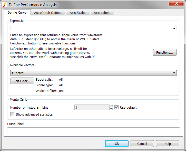
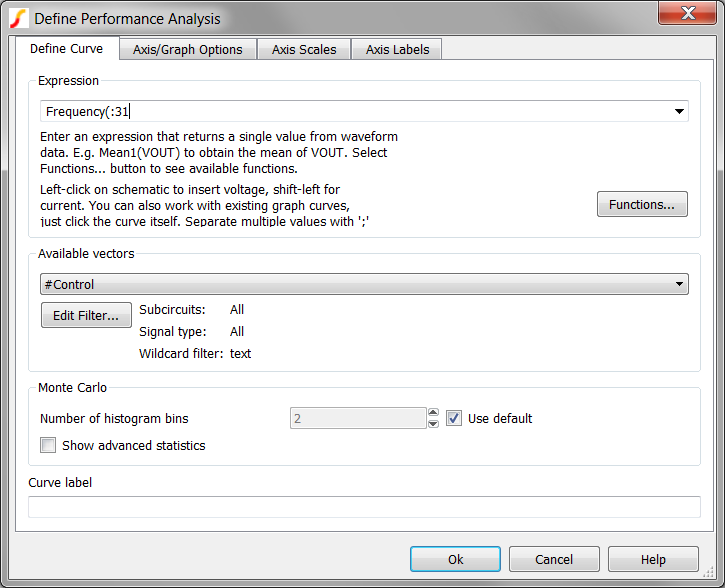
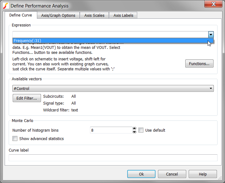
- From the schematic menu, select .Result: The Define Performance Analysis dialog opens:
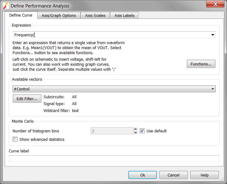
- In the Expression field, type Frequency( and leave the cursor
positioned immediately after the opening parentheses.Result: The configured dialog should appear as follows. Note the cursor is placed immediately after the opening parentheses. The position of the cursor is important for the next step!
- On the schematic, move the mouse over to the output of the POP Trigger schematic
device.
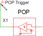
- Click the left mouse button once.Result: The POP Trigger output net, :31, is copied to the Define Performance Analysis dialog:
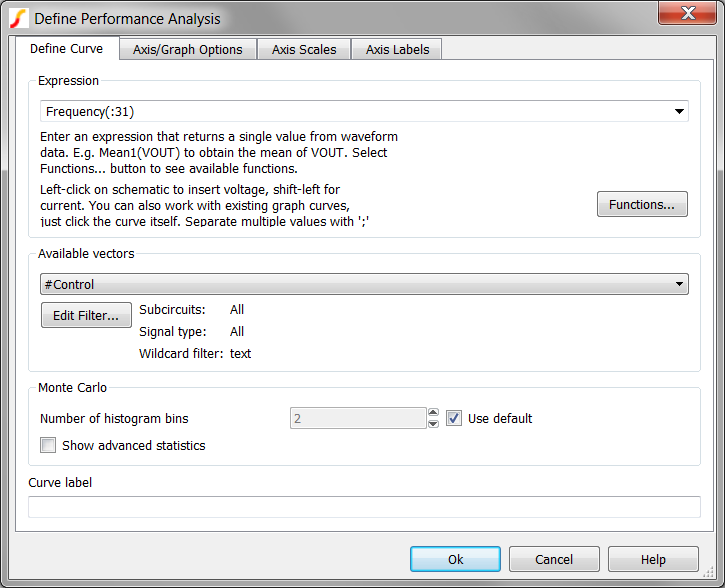
- Type a closing parenthesis ).Result: The final configured dialog should appear as follows: The final expression is Frequency(:31).
- The default number of histogram bins is defined by the equation:
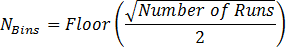 , which for a 32 run simulation will result in only 2 bins. For this
exercise, you will change the number of histogram bins on the Define Performance
Analysis dialog to 8. To change the number of histogram bins, follow these
steps:
, which for a 32 run simulation will result in only 2 bins. For this
exercise, you will change the number of histogram bins on the Define Performance
Analysis dialog to 8. To change the number of histogram bins, follow these
steps:- Uncheck the Use default checkbox.
- Enter 8 in the Number of histogram bins field.
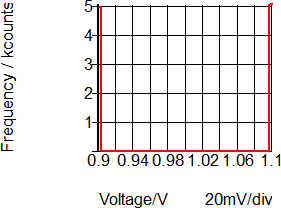
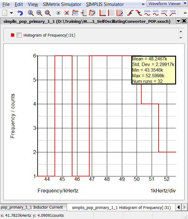
- Click Ok.Result: The histogram for the frequency of the converter is output to the waveform viewer:
Some Histogram Tips and Tricks
- The Define Performance Analysis dialog remembers previously plotted expressions.
If you execute the schematic menu , you can access the previous expressions with the pull down menu as
depicted below. This will save you time if you wish to re-plot a histogram.
- A list of functions which can be used to define the histogram expression is available by clicking on the Functions... button.
- More information on using this dialog to generate plots is available by clicking on the Help button.
Monte Carlo Log File
- The parameter name and default value.
- The evaluated parameter value and the percentage deviation from the default value.
- The seed value which was used to create this particular set of parameter values.
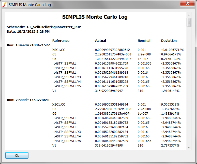
The log file is automatically created as a plain text file which can be opened in a spreadsheet program or otherwise machine parsed. A human-readable log file can be viewed using the . A sample log file appears as follows:
Monte Carlo Seed Values
Behind the scenes, a pseudo-random number generator is used to generate the Monte Carlo seed values. The seed values are used by each statistical probability function to generate the function return value. As a result, a particular Monte Carlo step can be repeated if you know the seed number used for that step, and the circuit has not changed at all between the first and second runs.
In the next exercise you will find the run with the lowest frequency and it's seed number, then repeat a simulation using the seed value.
Exercise #5a: Find the Run Number Which Produced the Lowest Frequency
On the waveform viewer window:
- Select the transient waveform tab if the histogram is the current tab.
- Press the keyboard shortcut C to turn on the cursors.Result: A hint box may open, depending on your preferences.
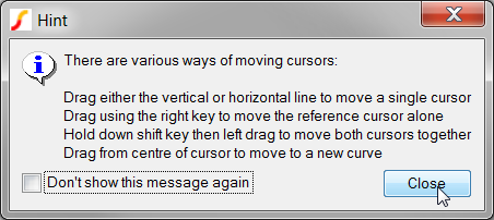
- Click on the Close button to dismiss the hint box.Result: The cursors are displayed on the graph.
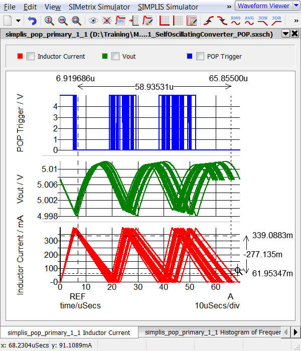
- There are two cursors, labeled REF and A. Move your mouse over the
A cursor until the cursor changes shape to a 4-way arrow as shown
below.
- Press and hold the left mouse button while moving the mouse to the right-hand most Inductor Current curve. This is the curve with the lowest frequency.
- Release the mouse button.Result: The cursor snaps to the nearest curve.
- If you moved the REF cursor in the previous step, repeat for the process
for the A cursor.Note: The exact cursor location on the curve is not important. What is important is the A cursor is on the right-hand most curve which is the step with the lowest frequency.
- From the graph menu, select .Result: the curve information, including the Monte Carlo run number is output to the SIMetrix/SIMPLIS command shell:
Curve name: Inductor Current (simplis_pop_primary_1_1)
Source group: simplis_pop_primary_1_1
Curve id : 17
Run number : 22
In this exercise, you have found the run number which produced the lowest converter switching frequency. In the next exercise, you will find the seed value and the simulated parameter values from the Monte Carlo Log file.
Exercise #5b: Find the Parameter Values Used for a Particular Run Number
You now know that run number 22 produced the lowest switching frequency. To find the seed value which corresponds to this run number, you open the Monte Carlo Log file. To open the Monte Carlo Log file, follow these steps:
- From the schematic menu select .Result: The Monte Carlo Log file opens.
- Scroll to run #22:
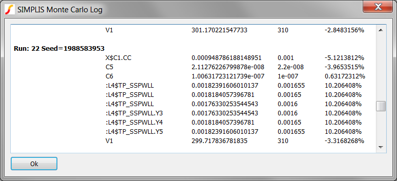
Note the seed value 1988583953 which was used for this run. In this converter, the switching frequency is highly dependent on the inductance value. Not unexpectedly, the evaluated parameter value for the inductance is higher than the default value, which requires longer charging and discharging times, and hence a lower switching frequency results.
In the next exercise, you will run a single step simulation using the same parameter values which generated the lowest frequency simulation run. You do this by running a Monte Carlo simulation using the seed value found in this exercise.
Exercise #5c: Run a Single Step Using a Known Seed Number
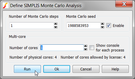
- From the schematic menu, select .Result: The Define SIMPLIS Monte Carlo Analysis dialog opens with the Monte Carlo configuration information.
- Make these three changes to the dialog values:
- In the Monte Carlo Seed field, paste the seed value: 1988583953
- Change the Number of steps to 1
- Change the Number of cores to 1Result: The configured dialog should appear as follows:
- Click Run to run the known seed value of 1988583953.Result: A single Monte Carlo Step is run, reproducing the Monte Carlo run with the lowest frequency:
- Press the Home key on the keyboard to zoom the waveform viewer to see the
full waveforms:
Exercise 6: Run DVM Monte Carlo
All actions described in this topic can be automated using the Design Verification Module (DVM). For example, the input voltage source value can be modified to use a statistical distribution function before launching a Monte Carlo simulation. DVM then launches the Monte Carlo simulation and as an additional feature, captures the fixed probe measurements and saves these measurements to a HTML formatted report file.
In this exercise you will run a 32 step Monte Carlo simulation using DVM and as in exercise #5 you will determine the worst case minimum switching frequency. As discussed in the SIMPLIS Mutli-Step Analysis, DVM requires a prepared schematic and a testplan. The schematic used in the previous topic will also work for DVM Monte Carlo, so the only other item is the testplan. A testplan with a single Monte Carlo test is shown below. The single test takes the schematic, changes the V1 value to {310*Unif(0.0333)}, and launches the Monte Carlo test with the values the user entered in the DVM Control Panel.
| *** | ||
| *** 3.2_monte_carlo_basic.testplan | ||
| *** | ||
| *?@ Analysis | Change( V1.VALUE , {Vin} ) | Label |
| *** | ||
| MonteCarlo | {310*Unif(0.0333)} | DVM Monte Carlo |
To run a DVM Monte Carlo simulation, follow these steps:
- Open the 3.2_SelfOscillatingConverter_POP_DVM_basic.sxsch schematic.
- On the schematic, double click on the DVM Control Symbol:
 Result: The DVM Control Panel Dialog opens.
 - Select the Monte Carlo Analysis item from the list on the left hand side of
the dialog.Result: The Monte Carlo Analysis parameters come into view. This is where you will enter the Monte Carlo parameters used in DVM simulations. These parameters override any parameters you set using the menu.
- Click Cancel on the DVM Control Panel dialog.
- From the menu bar, select .Result: A file selection dialog opens.
- Select the testplan named 3.2_monte_carlo_basic.testplan, and click Ok.
- Select the only test in this testplan:
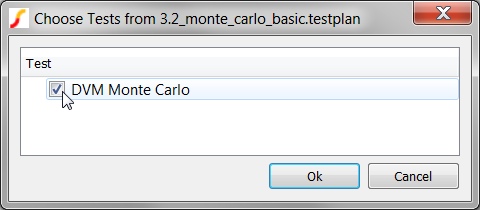
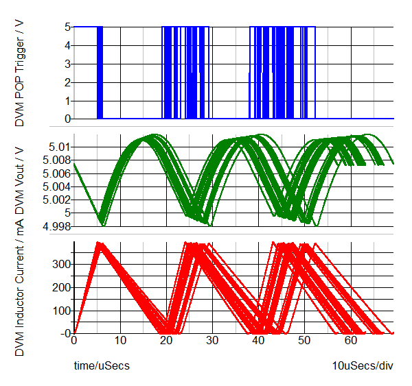
- Click Ok.Result: DVM changes the value of the input source, creates the Monte Carlo configuration file from the testplan, and outputs the following curves before opening the report.
The Monte Carlo DVM Report contains all the seed, parameter, and scalar measurement data taken from the simulation run. This table shows the seeds and measured values.
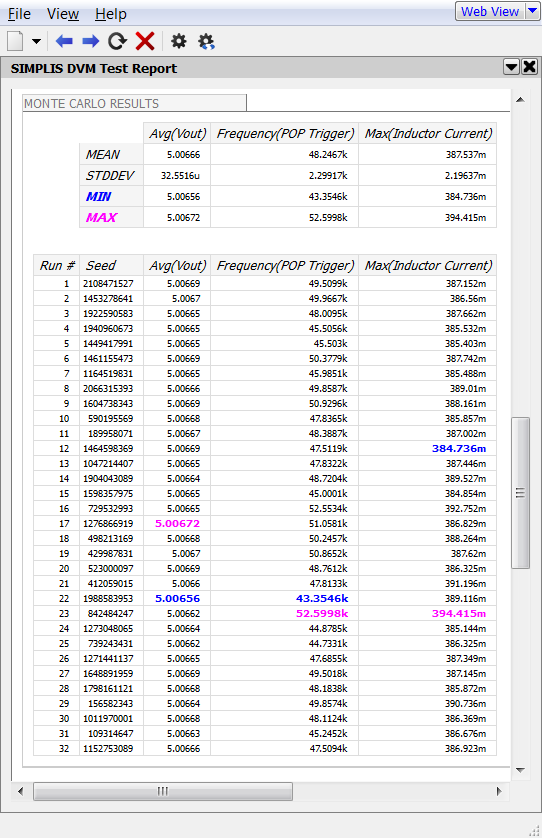
Note that run #22 is the simulation with the lowest frequency. It should be pointed out that DVM doesn't produce different results than a ordinary SIMPLIS Monte Carlo simulation. Instead, DVM automates the process of setting up the schematic and collecting the results into a HTML formatted report.
Conclusions and Key Points to Remember
- Setting up a SIMPLIS Monte Carlo Analysis is similar to a SIMPLIS Multi-Step Analysis; however, instead of stepping a parameter, the Seed value is stepped.
- The Gauss(), GaussTrunc(), Unif(), and Wc() probability distribution functions allow you to vary parameters during a Monte Carlo Analysis.
- Matched parameters can be defined by first defining a master variable in the command (F11) window.
- Histograms are easily plotted using the schematic menu: .
- The seed values used for a SIMPLIS Monte Carlo Analysis are saved to the Monte Carlo log file.
- Any single seed value can be simulated to reproduce a run with unusual or otherwise interesting results.