4.5 Add Scalar Measurements to Probes
This section of the tutorial describes how to automatically make the measurements described in 4.4 Add Scalar Measurements to Output Curves after a simulation completes by adding the measurements to the fixed probe symbols.
Any built-in or user defined measurement can be added to the fixed probes on the schematic. Measurements added to the probes are then automatically executed after each simulation run with the scalar measurement output to the waveform viewer and optionally to the schematic. The full version of SIMetrix/SIMPLIS has this feature enabled by default. This feature is available in SIMetrix/SIMPLIS Intro for a time-limited period using the Unlock Features option.
In this topic:
Key Concepts
This topic addresses the following key concepts:
- The built-in measurements can be added to any fixed probe.
- Measurements assigned to probes will automatically be made after the simulation completes.
- One or more measurements can be added to multiple probes by selecting the probes and running the context menu Edit / Add Measurement....
What You Will Learn
In this topic, you will learn the following:
- How to add measurements to fixed probes.
- How to add the same set of measurements to multiple probes.
4.5.1 SIMetrix/SIMPLIS Intro Users : Unlock Probe Measurements
To unlock the probe measurement feature, follow these steps:
- From the menu bar, select .Result: The Get Unlock Code window appears.
- Click the Unlock button.Result: A message returns indicating that the feature has been unlocked and that you must restart SIMetrix/SIMPLIS.
- Close and restart SIMetrix/SIMPLIS.
4.5.2 Adding Fixed Probe Measurements
To add fixed probe measurements to the schematic, follow these steps after reopening the last schematic. A copy of the schematic can be downloaded here: 8_SIMPLIS_tutorial_buck_converter.sxsch.
- In the Schematic editor, click on the probe with label VOUT; then right click
and select Edit / Add Measurement... (or use the keyboard shortcut
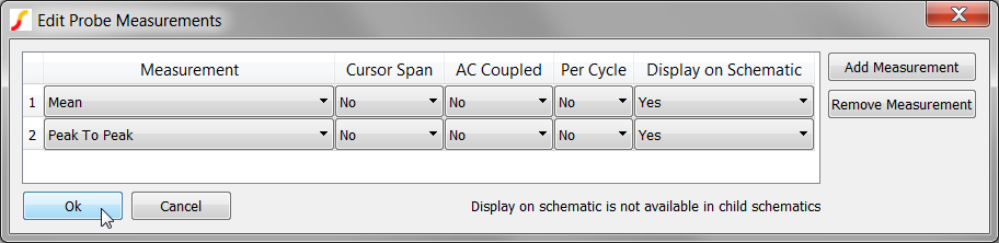
Ctrl+Alt+F7).Result: The Edit Probe Measurements dialog appears.
- From the Select Measurement drop-down list in the first column, select Mean.
- Click the Add Measurement button on the right and then select Peak To Peak as the second measurement.
- In the fifth column, Display on Schematic, select Yes for both Mean and Peak to Peak.
- At the bottom of the dialog, click Ok to save the probe measurements.
- In the Schematic editor, select the IL probe, type Ctrl+Alt+F7, and
repeat steps 2 and 3, adding the Mean and Peak to Peak measurements,
and then click Ok. Note: Since the default for Display on Schematic is No, no additional changes are needed on the IL probe nor on the SW probe.
- Return to the Schematic editor, click the SW probe, type Ctrl+Alt+F7, add Minimum and Maximum measurements, and then click Ok.
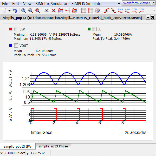
- If the waveform viewer is open, close it and press F9 to run the simulation.
Result: The schematic is updated with the VOUT curve measurements, and the graph now appears with the measurements for all three curves. You may have to drag the splitter bar just above the tabs in the waveform viewer to see all the measurements.
4.5.3 Saving your Schematic
To save your schematic, follow these steps:
- Select .
- Navigate to your working directory where you are saving your schematics.
- Name the file 9_my_buck_converter.sxsch.
A schematic saved at this state can be downloaded here: 9_SIMPLIS_tutorial_buck_converter.sxsch.