SIMPLIS - Piecewise Linear, All the Time
In SIMPLIS, all nonlinear device characteristics are modeled using a sequence of piecewise linear (PWL) straight-line segments. Consequently, SIMPLIS behavioral models for such devices differ from the corresponding SPICE models, which often seek to map device physics to device characteristics. Because the entire SIMPLIS system is made up of PWL device models, the set of system equations that SIMPLIS solves is also piecewise linear. While the topology and values in this system of equations can change radically at any time, SIMPLIS is solving a linear system of equations at every individual step. The result is that SIMPLIS can solve its set of system equations much faster and more accurately than can be done, in practice, with the SPICE approach. The speed and accuracy with which SIMPLIS solves for each change in the PWL system equations is a key reason that SIMPLIS can be effective in addressing the simulation challenges of power electronic systems.
The next section provides a brief, but important, overview of PWL modeling and demonstrates the level of accuracy versus laboratory measurements that can be routinely attained.
SIMPLIS Piecewise Linear Modeling Techniques - Overview
SIMPLIS is based on piecewise linear (PWL) modeling that approximates non-linear device characteristics using a series of piecewise linear straight-line segments. Although more PWL straight-line segments achieve higher accuracy, more PWL segments also can result in longer simulation times. The goal of PWL modeling is to achieve the desired level of accuracy while consuming the least amount of CPU time. SIMPLIS rewards the user who adds only the degree of complexity required for each device model to achieve the needed level of accuracy.
New SIMPLIS users often assume that piecewise linear modeling of power electronic systems must, by its very nature, be a crude approximation of reality. This is not the case for most switching systems. In fact, from the practical point of view of how much modeling and simulation effort are required to obtain a given level of accuracy in simulation results, PWL modeling often proves to be superior, allowing engineers to analyze systems with a complexity that would, otherwise, exceed the practical reach of a typical SPICE modeling approach. The key is to concentrate model complexity where it provides the most contribution to accurate results. Typical SIMPLIS PWL simulation results, when compared to laboratory measurements, demonstrate the high level of accuracy that is achievable using the PWL modeling techniques.
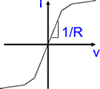
The table below illustrates how SIMPLIS represents PWL resistors, PWL capacitors, and PWL inductors as a set of PWL straight-line segments. A PWL resistor is piecewise linear in the current versus the voltage plane. The slope of this curve is the conductance. SIMPLIS automatically extends the left-most and right-most PWL segment to negative and positive infinity, respectively.
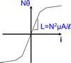
PWL capacitors are defined on the charge versus voltage plane where the slope is capacitance. PWL inductors are defined on the flux-linkage versus current plane, where the slope is inductance. The units of flux linkage are Weber-Turns or volt-seconds.
| PWL Resistor | PWL Capacitor | PWL Inductor |

|

|

|
|

|
|
| x-value ⇒ Voltage | x-value ⇒ Voltage | x-value ⇒ Current |
| y-value ⇒ Current | y-value ⇒ Charge | y-value ⇒ Flux Linkage |
| Slope=1/Resistance | Slope=Capacitance | Slope=Inductance |
An example schematic which demonstrates the PWL resistor, capacitor, and Inductor can be downloaded here: SelfOscillatingConverter_POP_AC_Tran.zip.
For detailed descriptions of the SIMPLIS primitive PWL models, see PWL Resistors.
Piecewise Linear Resistors
The forward transfer characteristics of a typical power diode is shown below. The red curve is from a SIMetrix-SPICE simulation and the blue curve is from a SIMPLIS simulation on a SIMPLIS PWL version of the same model.
This diode model example is a PWL resistor with three segments, automatically generated by the SIMPLIS model parameter extraction routine. This PWL diode model is good except around the knee of the diode curve. The illustration below is an example of concentrating model accuracy where it makes the highest contribution to the accuracy of the results.
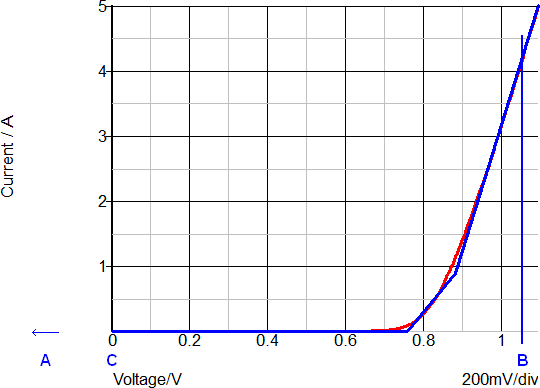
The simulation results for the above diode, which is used as a flyback converter rectifier, are shown in the set of curves below. The points A, B, and C note three different time instants during any switching cycle. The same points are noted on the forward transfer characteristics above. The three points are are listed in the table below.
| Time point | Description | Forward Current (A) | Forward Voltage(V) |
| A | Reverse biased | -22n ( -22V/100Meg ) | -22 |
| B | Forward biased | 4.1 | 1.1 |
| C | Zero biased | 0 | 0 |
Based on the transient waveforms, the diode is conducting (point B) or blocking (point A) for most of the switching period. In fact, in this circuit, the diode spends so little time in the knee of the diode curve where the device model is less accurate, that the system behavior can be accurately simulated despite the three-segment PWL model approximations. In switch-mode power conversion, rectifying diodes are often rapidly switched from a conducting to a blocking state. Using a PWL resistor model for these diodes can produce accurate results because very little time is spent operating in the region where the model fidelity is weaker.
On the other hand, if the same diode was used in an analog multiplier circuit where the exponential nature of the forward transfer characteristics is exploited, the results will have poor simulation accuracy because a three-segment PWL model does not adequately represent the exponential diode-current versus voltage characteristic.
Piecewise Linear Capacitors
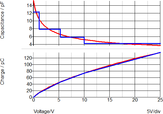
A good example of a PWL capacitor application is the junction capacitance of a diode. The same diode used in the PWL resistor example can optionally have a PWL capacitor included to model the junction capacitance of the device. By selecting a Level 1 model, the diode includes a four-segment PWL capacitor with the capacitance values determined by the SIMPLIS model parameter extraction routine.
The curves below show the capacitance and charge versus the reverse voltage for the diode in this example. This model uses a four-segment PWL capacitor to model the junction capacitance of the diode. On the upper graph, the red curve shows the continuous capacitance change of the SPICE model with reverse voltage. The blue curve shows the SIMPLIS step-wise constant capacitance versus reverse voltage curve.
The lower graph shows the charge versus reverse voltage with the SPICE model in red and the SIMPLIS model in blue. Although the error between points on the capacitance curve is often large, the error between the two charge curves is small. In most switch-mode applications, the total capacitive charge versus voltage characteristic is the dominant factor in determining device transitions from a conducting state to a blocking state and vice-versa. Consequently, PWL capacitors can be used to accurately represent junction capacitances in switch-mode power conversion applications.
Piecewise Linear Inductors
The saturation effects of inductors and transformers are important elements in switch-mode power conversion. SIMPLIS offers an easy way to model the saturation of an inductor or transformer by using a PWL inductor. In the circuit example, SelfOscillatingConverter_POP_AC_Tran.zip, the transformer is composed of an ideal DC transformer TX2 in combination with a magnetizing inductance L4, Leakage inductance Lleak, and winding resistances RW1, RW2, and RW3. The saturation of the transformer is determined by the PWL definition of L4. In the schematic image below, the components highlighted in blue below represent the transformer.
The transformer in this example has a magnetizing inductance made up of three PWL segments.
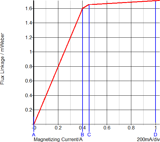
- The normal, or non-saturated, inductance 1.6mWeber/0.4A or 4mH.
- The first saturating section of the inductor comes when the inductor current is between 0.4 and 0.45A. The inductance in this region is (1.65m-1.6m)/(0.45-0.40) or 1mH.
- The final PWL segment represents a "hard" saturation. The inductance of this segment is 100uH.
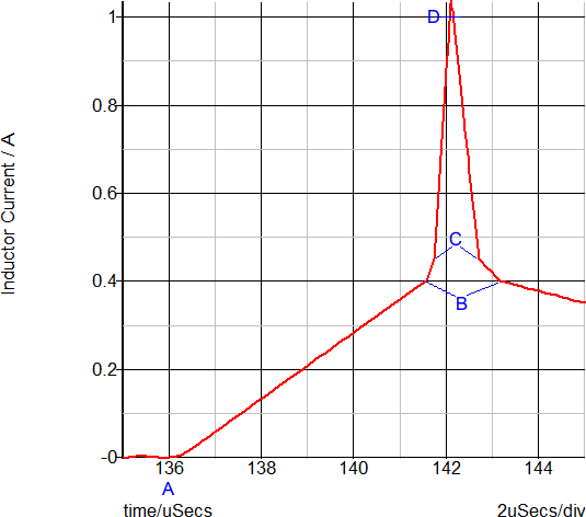
During the transient simulation, a load step is applied at 100us. The converter then enters an overloaded condition where the output voltage drops and the transformer enters into saturation. In the following graph, the load step is green and the inductor current is red.
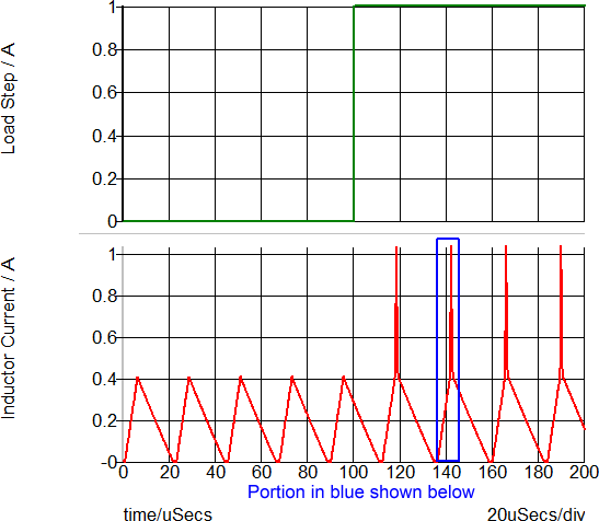
This overload condition shows the transformer saturation and how the PWL inductor closely represents a saturating inductor. The following two graphs show a close-up view of the time-domain waveforms and the current-flux linkage plane on which the PWL inductor is defined. The three PWL inductor segments can be seen in both the transient and in the x-y plot of the current-flux linkage plane.