Generating Efficiency Plots with Multi-Step Runs in DVM
In the previous section, DVM Principles, you learned the rules and principles of DVM, including some of the allowed testplan entries. In this topic you will run the testplan you examined in the DVM Principles topic on a converter and view the HTML report output.
To download the examples for the Applications Module, click Applications_Examples.zip
In this topic:
Key Concepts
- Multi-Step simulations, even when run on a single core, are much faster than single step simulations because the schematic is prepared for simulation once.
- Multi-Core Multi-Step simulations only compound the speed up effect - allowing you to run many simulation steps in a short period of time.
- The default parameter values for a particular test objective are taken from the DVM Control symbol. Values passed in the testplan overwrite these values.
- The CreateXYScalarPlot() function is an extremely powerful function which plots scalars against each other.
- Often a post process script is called during a NoSimulation test objective to analyze the results from all previously run tests.
What You Will Learn
In this topic, you will learn the following:
- How to run a custom testplan.
- How to change the stepped parameter range and step type.
- How to read and modify a post-process script.
Getting Started
To get started, open the schematic apps_d_1_llc_converter_efficiency.sxsch. This schematic is prepared to run DVM as described in the DVM Principles topic.
Exercise #1: Set the Number of Cores for the Multi-Step Simulations
The number of cores used in the multi-step simulations is determined by the value on the DVM Control symbol. In common with most simulation parameters, the number of cores can be overridden in a testplan entry. This is the way DVM works:
- Properties are read from the DVM Control symbol first,
- Second, optional overrides are checked in the testplan.
This is an extremely important concept - that default values are loaded from the DVM Control symbol, then user specified overrides are checked in each test in the testplan. In this case, the default number of cores is one and you will change this on your schematic to reduce the simulation time. The change the number of cores,
- Double click on the DVM Control symbol to bring up the editing dialog.Result: The DVM Control Symbol dialog opens to the Multi-Step page.
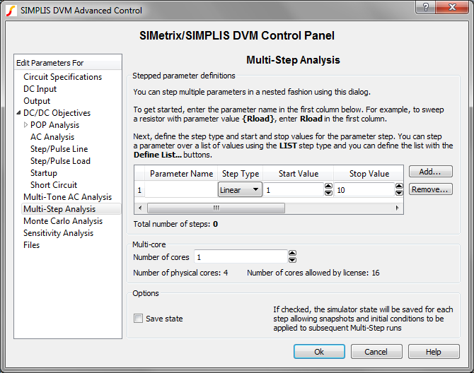
- Increase the number of cores to the maximum number allowed by your physical hardware or the license. This is typically 2 or 4.
- Click Ok.
Exercise #2: Choose and Run the Testplan
Now you are ready to run this testplan on the schematic. To run the testplan,
- Select the .Result: A testplan file selection dialog opens.
- Navigate to the testplans directory
- Choose the apps_d_1_llc_converter_efficiency.testplanResult: The test selection dialog appears with the two tests defined in the testplan.
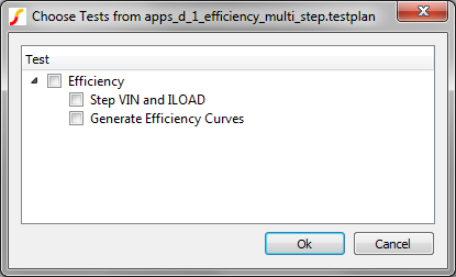
- Check the first box in the dialog, to the left of the Efficiency
text.Result: Both tests are selected to be run. The text in the test selection dialog is determined by the Label in the testplan with hierarchy delineated with the pipe "|" character. You can select and deselect all tests in a hierarchical path by selecting the parent checkbox.
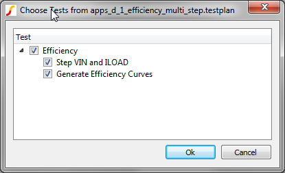
- Click Ok.Result: DVM starts on the first selected test, configuring the schematic for the nested Multi-Step simulation with the Steady-State test objective. After about a minute, DVM moves onto the second test which generates the summary curves. The overview report opens in SIMetrix/SIMPLIS.
Exercise #3: Examine the Test Report
The test report consists of two different types of HTML pages:
- The Overview report which has hyperlinks to each individual test report.
- The individual test reports which detail the results from the tests.
By default, when you run two or more tests, the overview report is displayed. In addition to the hyperlinks to the individual test reports, the overview report has provisions for overview graphs like the efficiency graph, and overview scalars, which are not present in this report.
DVM makes a number of scalar measurements and also captures each probe measurement for any probe with a name prefixed with DVM. Also, in the html report you will only see curves which you have named to start with DVM - all other curves are suppressed from the images in the reports. These curves are retained for each graph file for which there is a hyperlink under the graph image in the report.
All scalar values are presented in table form in the report, and tab delimited text files summarizing the scalar values are generated as well.
Exercise #4: View the Post-Process Script
A great deal of the "magic" happens in the post process script. While you are not expected to be an expert in scripting, this exercise will help you understand how you can take a script from the training course material and modify it for your application. To get started,
- Navigate back to the schematic by clicking on the tab.
- On the File Viewer, click on the Sync to Active button.Result: The file viewer opens to the directory which contains the schematic.
- Click on the arrow in front of the scripts directory.Result: The scripts directory opens.
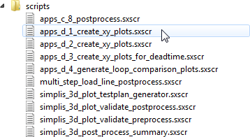
- Double click on the apps_d_1_create_xy_plots.sxscr entry.Result: The script opens in the internal editor.
The Arguments to The Script
The first non-comment line in the script is on line #5:
| 5 |
Arguments @retval label report_dir log_file controlhandle |
This line defines the script arguments - these arguments are fixed and will be the same for all scripts which are called from a preprocess or postprocess script in DVM.
The Logical Test
The next non-comment line is on line #9, where the script performs a logical test on the currently executing test label. The label is passed into the script from the testplan entry and the post process script uses this label to decide what actions to take. In this case, the logical test is on line #9:
| 9 |
if StrStr( label , 'Generate Efficiency Curves' ) > -1 then |
searches the text label for the string Generate Efficiency Curves, and if that string is found, the script proceeds to generate the efficiency curves. The StrStr Function is built into SIMetrix/SIMPLIS.
The Input Voltage Variable
Assuming the logical test passes, the script next assigns the input voltage steps on line #15:
| 15 |
Let vins = [ 360 , 380 , 400 ] |
This is a real array or a vector with three elements. In the next section of the script, a "for" loop will loop over each of these three elements and create curves for each of the input voltages.
The For Loop
Next, the script loops over the three input voltages with a "for" loop, on line # 17:
| 17 |
for i = 0 to length( vins ) - 1 |
The CreateXYScalarPlot() Call
Inside the for loop is a single executable line - this line calls the incredibly powerful CreateXYScalarPlot() function. This function reads scalar values from all previous tests and plots mathematical expressions of those scalar values on an X-Y plot. In order to accomplish this high level of functionality in a single function, the CreateXYScalarPlot() function has two arguments, with the first argument having 7 or 8 elements.
The arguments to the function are all strings. Strings in the script language are denoted by enclosing the string text inside single quotes. In order to make it clear which element is which, the first argument is spread out with one element per line. Each continued line begins with the plus "+" character to denote the line is a continuation of the previous line. Using this format allows for easier error detection in case the function fails to create the curve.
The elements which compose the first argument are described with comments in the script. The actual function call starts on line #30 and continues through line 39:
| 30 | Let return = SimplisDVMAdvancedUtilMeasurementCreateXYScalarPlot( [ | |
| 31 | + 'ILOAD', | |
| 32 | + 'Efficiency_WHEN_VIN_' & vins[i] , | |
| 33 | + 'Efficiency_WHEN_VIN_' & vins[i] , | |
| 34 | + 'DVM Efficiency VIN ' & vins[i] & 'V' , | |
| 35 | + 'DVM Efficiency vs. ILOAD', | |
| 36 | + 'A1', | |
| 37 | + 'vert' , | |
| 38 | + 'usescalars=multi xlabel=Load Current xunits=A ylabel=Efficiency yunits=%%% showpoints=true color=SEQ:' & i + 1 ], | |
| 39 | + log_file ) |
The line-by-line analysis of this function call is as follows:
Line 30 - starts the function call with a Let command, followed by the function name. This line starts the first argument as an array with a square opening bracket "[".
Line 31 - The x-axis expression. You can combine any scalar values in a mathematical expression in this element.
Line 32 - The y-axis expression. As with the x-axis expression, you can combine any scalar values in a mathematical expression in this element.
Line 34 - The name of the resulting curve. You must prefix this with DVM or the curve will not appear in your output report.
Line 35 - The Graph name, again this should start with DVM.
Line 36 - The analog axis to place the curve on. "A1" is the first (lowest or default) axis, 'A2' is the next axis and so on.
Line 37 - The axis alias - only used when A1 is used for multiple axes.
Line 38 - The "Optional Parameter String." DVM uses optional parameter strings to pass information to functions, both in the testplan and in the script functions. These optional parameter strings are space delimited strings of parameter name=parameter value without spaces on either side of the equals sign. In this function the optional parameter string labels the graph axes, the curve color, etc.
Line 39 - This is the second argument to the function and is always the log_file variable which is passed into the script from DVM.
Promoting the Graph to the Overview Report
After the for loop creates all the curves on the new graph, a call to the PromoteGraph() function tells the program to feature the graph on the overview report. The PromoteGraph function has several forms, the one used on line #44:
| 44 | Let return = SimplisDVMAdvancedUtilMeasurementPromoteGraph([ 'DVM Efficiency vs. ILOAD' , '200' ], log_file) |
applies a weight of 200 to the graph. Graphs on the overview report are displayed in the order of highest to lowest weighting.
Conclusions and Key Points to Remember
- Using the Multi-Step analysis on two stepped parameters in DVM allows you to quickly analyze a circuit's performance over line and load variations.
- Applying Multi-Core capability to the simulation results in even faster simulation times.
- The CreateXYScalarPlot() function generates X-Y plots from previously generated scalar values. This function saves time by automatically plotting the scalar results.