DVM Principles
In this topic, you will learn the terminology used in DVM and the principles governing the application of DVM to your designs. There are very few rules, but those rules which exist are non-negotiable and you will have to live by these rules in order to use DVM.
To download the examples for the Applications Module, click Applications_Examples.zip
In this topic:
Key Concepts
This topic addresses the following key concepts:
- To use DVM you need a schematic and a Testplan.
- Testplans are nothing but tab-delimited ASCII text files which you edit in a spreadsheet program.
- Each row in a testplan is a test to be executed, each column defines an action for that test.
- Testplans can use Symbolic Values which greatly simplify the reuse between schematic designs.
- When using symbolic values, the schematic stores the numerical values on the DVM Control Symbol and the testplan refers to those values using symbolic references.
- DVM uses special DC Input Sources, AC Line Input Sources, and Output Load symbols where the electrical subcircuit used in the simulation can be changed for each test in the testplan.
- DVM keeps track of these special source and load symbols with a system of Managed Sources and Loads.
- The 3 and 4 pin output load subcircuits include the AC perturbation source for a Bode Plot analysis.
- Objectives are pre-defined test
configurations which define:
- The source and load subcircuits.
- The analysis type, e.g. Transient, POP, AC.
- The post-simulation measurements to be make as well as any additional curves to create.
- Specialized analyses such as Multi-Step Analysis or Monte Carlo Analysis modify the test objective, by looping over a set of parameter values or by varying the seed value.
- Scalar measurements made by DVM can be selected on the DVM Control Symbol dialog.
- Curve post processing functions allow you to:
- Generate XY Plots such as efficiency vs. load current from scalar values measured in previous tests.
- Create a graph of Summary Curves by extracting curves from previous tests to a current test.
- Generate Bode Plots between any schematic nodes in the hierarchy.
- Generate curves from arbitrary expressions of schematic nodes.
What You Will Learn
In this topic, you will learn the following:
- How to configure a schematic for DVM.
- The basics of testplan syntax.
- The mechanics of setting up a test sequence with DVM.
DVM Slideshow
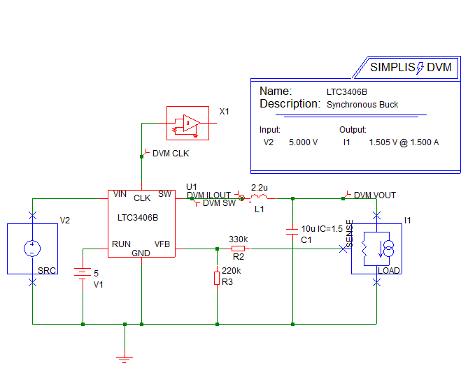
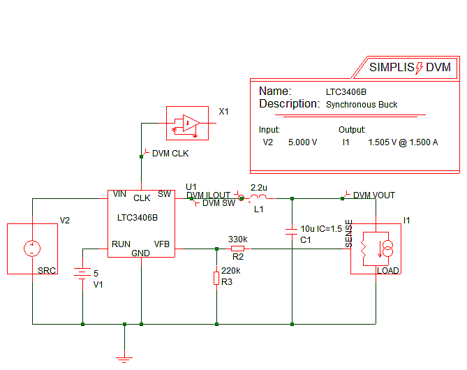
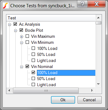
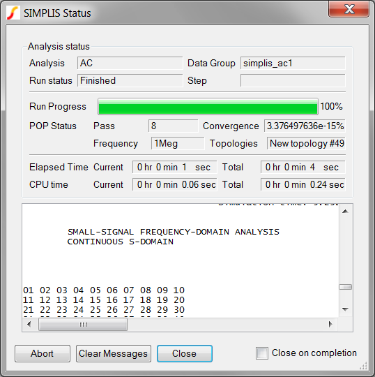
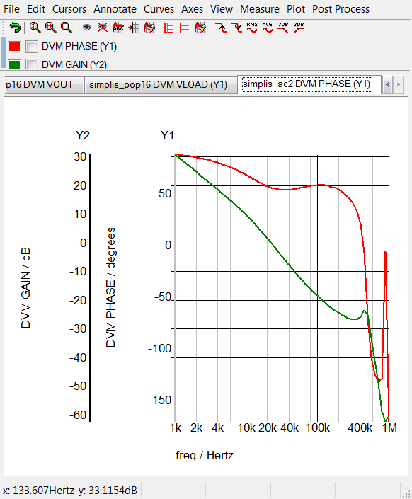
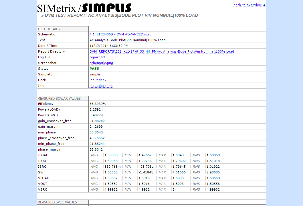
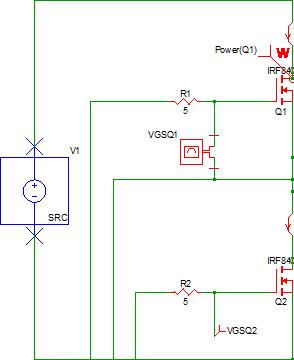
The following slideshow illustrates the sequence of actions that DVM takes as it executes a single test from the Built-In Sync Buck testplan. The test used for this example is the same BodePlot test described in the previous section.
- You can pause the slideshow by moving the mouse cursor over the images.
- To go forward or back one slide, click the arrow links that appear when you mouse over the slideshow.
- Each slide number is shown in the bottom right-hand corner. You can jump to a particular slide by clicking one of the gray squares at the bottom on the image. The current slide is indicated by the white square.
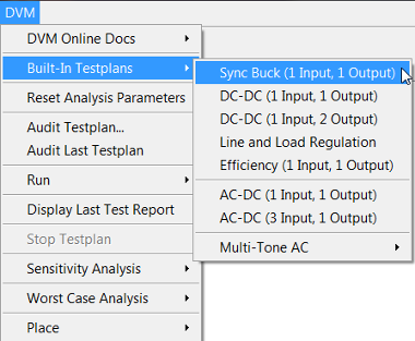
Although the slideshow illustrates actions that DVM takes for a single test from the built-in testplan, the DVM functionality encompasses much more than just Bode plot testing. Built-in testplans for one-input, one-output and one-input, two-output DC/DC converters are provided and include a full suite of tests that designers often run on power supplies, including Step Line, Step Load, Input and Output Impedance, and more.
Additionally a full suite of AC/DC tests are available in the one-input, one-output and thee-input, one-output Built-In AC/DC testplans.
For a full list of available tests, see the the following topics:
DVM also provides the ability to customize testplans to suit any design. For details about how to customize test plans, see Customizing Testplans in the DVM Tutorial.
Part I: Preparing the Schematic for DVM
At the very minimum, preparing a schematic for DVM requires you add the basic DVM control symbol. This symbol doesn't store the Symbolic Values for the input voltage range or full load current; therefore, schematics using this symbol cannot run the built-in testplans which use the test Objective testplan entries. For this reason, the basic DVM Control Symbol has limited functionality and will not be used in this course.
- A DVM input source and an output load symbol.
- A DVM Control Symbol.
- You to entering the design specifications for the input voltage and output load into the DVM control symbol.
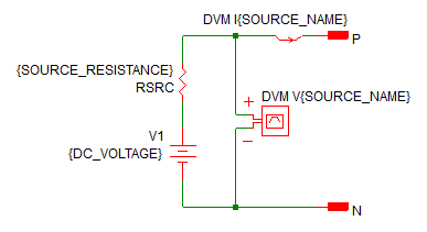
Exercise #1: Add an Input Source Symbol
To add the input source, follow these steps:
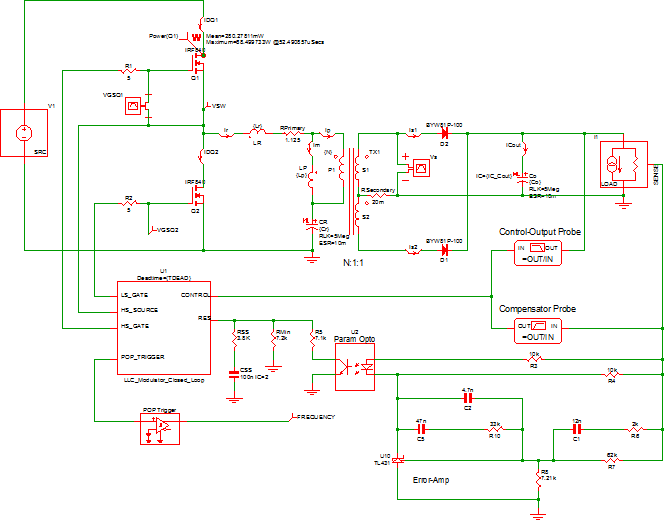
- Open the apps_d_0_llc_converter_efficiency.sxsch.
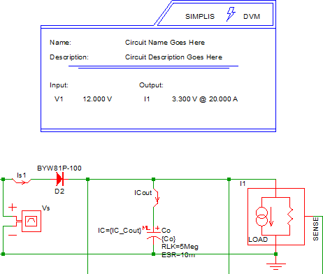
- Delete the DC voltage source VIN on the left side of the schematic.
- From the parts selector, choose , and place the symbol where you removed the DC source VIN.
- Add and remove wires to connect the source as shown below:
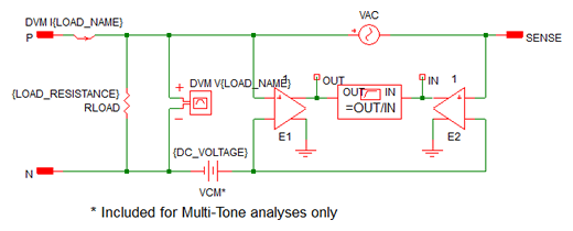
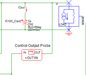
Exercise #2: Add a 3-Terminal Output Load Symbol
The 3 and 4-terminal DVM output loads have a SENSE (3-terminal) or a differential SENSE (4-terminal) connection. These extra pins allow DVM to include the injected AC perturbation source and Bode plot probe that are required for closed-loop AC analysis. DVM automatically inserts these components into the load subcircuit definition for the Bode plot tests. For this circuit you will use the 3-terminal output load.
To add the 3-terminal output load, follow these steps:
- Delete the RL resistor and VAC source from the right side of the schematic.
- From the parts selector, choose , and place it where you removed the load resistor RL. You will need
to mirror the symbol about the vertical axis using the F6 key before
placing the symbol.
- Connect the SENSE terminal on the DVM 3-terminal output load to the
feedback network. Note: The SENSE terminal provides the output voltage feedback information to the converter control loop. During Bode plot tests, the small signal AC source is inserted between the positive load terminal and the SENSE terminal and perturbs the control loop. For all other test objectives, the SENSE terminal is shorted to the positive output terminal of the load. The schematic should appear as shown below:
Exercise #3: Add the DVM Control Symbol
To place a DVM control symbol, follow these steps:
- From the parts selector, choose .
- Place the symbol at the top of the schematic.
It is important to note that when you place the DVM Control Symbol after placing the source and load symbols, DVM performs a number of housekeeping tasks. These include:
- DVM detects the input source and output load symbol(s) and configures the DVM Control Symbol accordingly. DVM supports up to five input sources and six output loads. You can add loads or sources at any time.
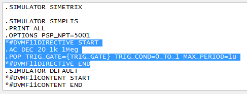
- DVM automatically reads the analysis parameters from the F11 window and adds these parameters to the DVM Control Symbol.
Exercise #4: Enter Circuit Specifications
The DVM control symbol has been configured with one managed input source (V1) and one managed output load (I1). When you placed the control symbol on the schematic with analysis directives already set from the dialog, these directives were copied onto the control symbol. Since the program has no way of knowing what the input and output voltages and load currents are, you need to change these parameters to suit this particular circuit.
To change the circuit specifications, follow these steps:
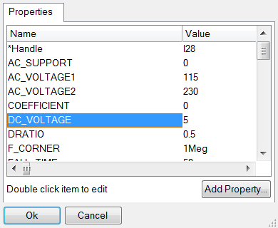
- Double click on the DVM control symbol. Result: The SIMetrix/SIMPLIS DVM Control Panel opens.
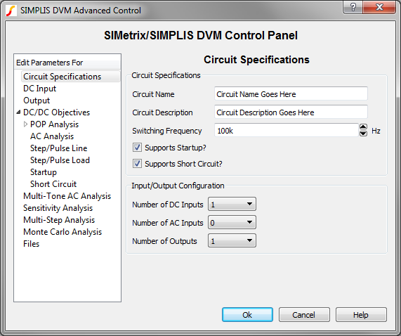
- On the Circuit Specifications page, set the values as listed in the following
table.
Parameter Value Units Circuit Name test_llc_converter Circuit Description LLC Converter Switching Frequency 85k Hz Note: Leave the default values for the other fields on this page. - Click on DC Input in the page-selection box on the left side of the
control panel, and then enter the values listed below.
Parameter Value Units Voltage Nominal 380 V Minimum 360 V Maximum 400 V Misc. Source Resistance 0 Ohm - Click on Output in the page-selection box, and enter the values listed
below.
Parameter Value Units Voltage Nominal 24 V Tolerances Peak to Peak 120 mV Current Maximum 5 A Light Load @ Vin Min 0.5 A @ Vin Max 0.5 A Note: Leave the default values for the other fields on this page. - Click on the POP Analysis entry to bring up the POP page.
- Verify that Use "Pop Trigger" schematic device is checked.
- Click Ok to save the specification changes.
- Save the schematic as test_llc_converter.sxsch.Result: At this point, the schematic is configured to run the built-in testplans which use symbolic values and the DVM source and load subcircuits. A pre-prepared schematic at this state is included in the zip archive with file name: apps_d_1_llc_converter_efficiency.sxsch.
Part II: All about Testplans
In the Key Concepts section you learned that to run DVM, you need a prepared schematic and a testplan to run on that schematic. In Part I you prepared your schematic for DVM, and in Part II you will learn about testplan syntax, and how to edit testplans.
- Blank lines are ignored.
- Lines starting with an asterisk (*) are considered comments and are ignored.
- Inline comments are not supported; that is, you can comment out an entire line, but not a portion of a line.
- Each non-blank, non-comment line in the testplan describes a set of test conditions for a single test. Each column performs some action during the test.
- The testplan can have a header row. The first entry on the header row starts with *?@. The program reads the file and identified the header row by looking for this special three character sequence.
- Any column can have an empty cell in a row but the behavior is different for columns
with function headings.
- If the column heading is a function, such as Var(vout , 1.2), DVM uses the default value, in this case 1.2.
- If the column heading is not a function, DVM makes no changes for that column where a cell is empty.
Exercise #5: Examine a Testplan
The best way to learn how to create and modify testplans is to look at a prepared testplan. In the Applications_Examples.zip file are a number of testplans. In the following sections you will use the apps_d_1_llc_converter_efficiency.testplan file.
The best program to view and edit testplan files is Microsoft Excel or a similar spreadsheet program. If you use one of these programs, be sure to save your file as tab delimited text, as DVM cannot read a Excel preadsheet file.
- Open the apps_d_1_efficiency_multi_step.testplan in Excel or a similar spreadsheet program.
- The spreadsheet has 7 rows and 9 columns:
| *** | ||||||||
| *** apps_d_1_efficiency_multi_step.testplan | ||||||||
| *** | ||||||||
| *?@ Label | Objective | Analysis | Analysis | Change( V1.DC_VOLTAGE , 380 ) | Change( I1.LOAD_RESISTANCE , 5 ) | Create | Create | Postprocess |
| *** | ||||||||
| Efficiency|Step VIN and ILOAD | Steady-State | Multi-Step( ILOAD , LIN , 10 , 0.5 , 5.0 ) | Multi-Step( VIN , LIST , 360 , 380 , 400 ) | {VIN} | {RLOAD} | Alias( Efficiency , Efficiency_WHEN_VIN_%VIN% ) | Alias( Efficiency , Efficiency_WHEN_ILOAD_%ILOAD% ) | |
| Efficiency|Generate Efficiency Curves | NoSimulation | ./scripts/apps_d_1_create_xy_plots.sxscr | ||||||
Let's examine the testplan row by row and then column by column. The first three rows are comments and are completely optional.
Comment Rows
| *** |
| *** apps_d_1_efficiency_multi_step.testplan |
| *** |
As long as the first character in the line is a *, you may change the text in these line without affecting DVM operation.
The Header Row
The next row is the extremely important header row. The header row tells the program what type of entries to expect in the following rows. It is assumed that all electrical tests are entered after the header row. Here is the header row and we will examine this in more detail:
| *?@ Label | Objective | Analysis | Analysis | Change( V1.DC_VOLTAGE , 380 ) | Change( I1.LOAD_RESISTANCE , 5 ) | Create | Create | Postprocess |
- The first entry:
*?@ Label
describes the test conditions. The Label is not electrically active and doesn't control the schematic configuration or measurements. It is simply there to provide the user an idea of the function of each test. - The second entry:
Objective
tells the program to expect one of the pre-defined test objectives. For example, there exists a BodePlot() Test Objective which measures the loop response of the circuit. - The third and fourth entries:
Analysis
can be used to modify the objective with a Multi-Step Analysis or other analysis types. Valid analysis entries are documented in the DVM Analysis topic. - The fifth and sixth columns change symbol property values. In this case, the property name and default value are defined in the header. For each test, you can assign a value in the column for that test. If you leave any field blank, the default value entered in the header will be used.
- The seventh and eight column headers:
Create
allow you to create scalars or curves after the simulation has completed. - The final header entry:
postprocess
allows you to run a post process script after the simulation completes. In section Generating Efficiency Plots with Multi-Step Runs in DVM, you will see how you can use the CreateXYScalarPlot() in a post process script to create efficiency plots in DVM.
A couple of comments are in order and some conclusions can be made from this testplan header row.
- A testplan can have more than one header entry of the same type - in this case there are two Analysis entries. DVM will process the duplicated entries from left to right in the testplan row.
- There are two types of header entries -
- Those without function notation, such as Label, Objective, Analysis, etc.
- Those which use function notation, for example, Change( V1.DC_VOLTAGE , 380 ).
FunctionName( argument1, argument2, …, argumentn )
This notation is common to several programming languages. The argument types, order, and minimum number of arguments are typically fixed by the function definition. The Change function takes two arguments, the first being the property address and the second, the property value. The property address is simply the reference designator and the property name separated by a period (.), so V1.DC_VOLTAGE tells the program to first find V1 and then change the DC_VOLTAGE property. - Although the testplan entries are processed from left to right, each type of testplan entry is processed in a particular order. For example, if you place the PostProcess entry first, it will still be run after the Analysis and Objective entries because the Analysis and Objective entries configure the schematic for the test.
The Multi-Step Test
Now that you understand how the header entries work, you will be able to understand the two tests which are on lines 6 and 7 of this testplan. The first test is on line 6:
| Efficiency|Step VIN and ILOAD | Steady-State | Multi-Step( ILOAD , LIN , 10 , 0.5 , 5.0 ) | Multi-Step( VIN , LIST , 360 , 380 , 400 ) | {VIN} | {RLOAD} | Alias( Efficiency , Efficiency_WHEN_VIN_%VIN% ) | Alias( Efficiency , Efficiency_WHEN_ILOAD_%ILOAD% ) |
As discussed previously, the label is non-electrical but hints that this test will measure the efficiency of the converter while stepping the VIN and ILOAD parameters.
The Objective is set to Steady-State. This test objective sets the input voltage source to a DC source and the output load to a resistive load. It then runs a POP analysis on the converter and by default makes the Efficiency measurement. Measurements can be added or removed on an objective by objective basis with the DVM Measurements dialog.
The Multi-Step( ILOAD , LIN , 10 , 0.5 , 5.0 ) and Multi-Step( VIN , LIST , 360 , 380 , 400 ) analysis entries step the ILOAD and VIN parameters using a nested multi-step simulation. You can add Analysis columns to step additional parameters. Although there is no practical limit to the number of parameters which can be stepped, the number of simulation steps increases geometrically as the number of parameters increase. In this example, the input voltage is stepped over three values and the load current over 10 values, making for a total of 30 simulation steps.
.VAR RLOAD = {24/ILOAD}
The next two entries use the Alias() entries. The Alias() function creates a copy of the scalar name in the first argument, in this case Efficiency, and renames the copy with the name given in the second argument, in this case Efficiency_WHEN_VIN_%VIN%. Notice the %VIN% in the new scalar name. This is a "template", and uses the same template replacement rules you learned in 5.1 Passing Parameters into Subcircuits Using the SIMPLIS_TEMPLATE Property. Since the VIN parameter is stepped over three values, 360, 380, and 400, three scalar names will be created:
- Efficiency_WHEN_VIN_360
- Efficiency_WHEN_VIN_380
- Efficiency_WHEN_VIN_400
Each of these scalar names will have 10 values, one for each of the ILOAD steps. This aliasing allows you to categorize scalars based on their stepped parameter value. In the next topic, Generating Efficiency Plots with Multi-Step Runs in DVM, you will see why this is concept is critically important.
The Final Test
In this testplan, the Multi-Step test runs 30 simulations, generating aliased scalars based on the stepped parameter values. In the final test, DVM is instructed to generate summary X-Y plots of these scalars, for example, plot Efficiency_WHEN_VIN_360 on the vertical axis and ILOAD on the horizontal axis. Here is where the power of scalar aliasing is exploited. By creating three scalar aliases, three curves, one for each of the minimum, nominal, and maximum input voltages can be plotted.
- The NoSimulation entry in the Objective column tells DVM not to run any simulation.
- The input source property DC_VOLTAGE is set to the default value of 380V.
- The output load property LOAD_RESISTANCE is set to the default value of 5A.
- The post process script apps_d_1_create_xy_plots.sxscr located in the scripts directory is called to generate the X-Y plots.
In the next topic : Generating Efficiency Plots with Multi-Step Runs in DVM, you will run this testplan and see how it can be modified for other applications.
Conclusions and Key Points to Remember
- Using DVM requires a schematic prepared for DVM, and a testplan defining the tests to be run.
- DVM can use symbolic values which are stored on the DVM control symbol.
- Testplans are simple tab delimited text files which you edit with a spreadsheet program.
- The header row defines the allowed entries in each test row - that is, the allowed column entries are defined by the header row entry for that column.