Multi-step Analyses
The analysis modes, Transient, AC, DC, Noise and Transfer Function can be setup to automatically repeat while varying some circuit parameter. Multi-step analyses are defined using the same 6 sweep modes used for the individual swept analyses in addition to snapshot mode. See Transient Snapshots for details of snapshots. The 6 modes are briefly described below. Note that Monte Carlo analysis is the subject of a whole chapter see Monte Carlo Analysis.
- Device. Steps the principal value of a device. E.g. the resistance of a resistor, voltage of a voltage source etc. The part reference of the device must be specified.
- Model parameter. Steps the value of a single model parameter. The name of the model and the parameter name must be specified.
- Temperature. Steps global circuit temperature.
- Parameter. Steps a parameter that may be referenced in an expression.
- Frequency. Steps global frequency for AC, Noise and Transfer Function analyses.
- Monte carlo. Repeats run a specified number of times with tolerances enabled.
- Linear
- Decade
- List
In this topic:
Setting up a Multi-step Analysis
Define Transient, AC, DC, Noise or Transfer Function as required then check Enable Multi-step and press Define... button. For transient/DC analysis you will see the following dialog box. Other analysis modes will be the same except that the frequency radio button will be enabled.
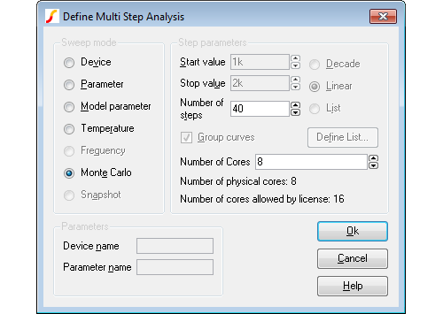
Enter parameter as described below. Only the boxes for which entries are required will be enabled. In the above example, only the Number of steps box is enabled as this is all that is required for Monte Carlo mode.
Sweep Mode
Choice of 6 modes as described above.
Step Parameters
Define range of values. If Decade is selected you must specify the number of steps per decade while if Linear is specified, the total number of steps must be entered. If List is selected, you must define a sequence of values by pressing Define List....
| Group Curves | Curve traces plotted from the results of multi-step analyses will be grouped together with a single legend and all in the same colour. For Monte Carlo analysis, this is compulsory; for other analyses it is off by default. |
| Number of cores | On multi-core computers, the work for multi-step analyses may be split between multiple cores to speed up the simulation. See Using Multiple Cores for Multi-step Analyses for more information. |
Parameters
The parameters required vary according to the mode as follows:
| Mode | Parameters |
| Device | Device name (e.g. V1) |
| Parameter | Parameter name |
| Model Parameter | Model name Model parameter name |
| Temperature | None |
| Frequency (not DC or transient) | None |
| Monte Carlo | None |
| Snapshot | See Transient Snapshots |
Using Multiple Cores for Multi-step Analyses
The work for multi-step analyses can be split between multiple processor cores to speed up the simulation. The maximum number cores that may be used is dependent on your license and on the number of processor cores that your system is equipped with. The speed improvement that can achieved by this method can vary due to a number of factors but is typically of the order of 75% of the core count. E.g. if you have 4 cores, the speedup may be about 3 fold.
Setting up a Multi-core Multi-step Simulation
Set up a multi-step simulation in the normal way but set the Number of Cores edit box to the number of cores you wish to use. You will not be able to set the number of cores to larger than a certain value depending on your system and your license. These values are shown below the number of cores selector.
Running a Multi-core Multi-step Simulation
Run the simulation in the normal way. The simulator status box will show a single entry for each core being used. See below
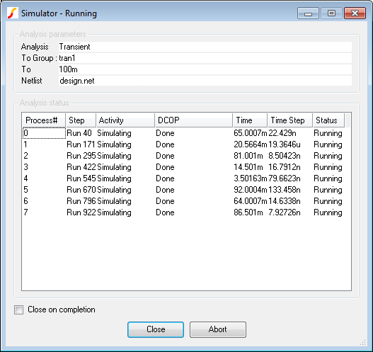
The above shows the status box showing for a 1000 step Monte Carlo analysis using 8 cores. Each line shows the status for each of the 8 processes. Apart from sending back status information, each of the 8 processes runs completely independently and writes to its own data file. When the run is complete the data from each processes will be linked to the main data file. Subsequently you can plot and analyse the results in exactly the same way as you would a single core run.
Using Fixed Probes with Multi-core Multi-step Simulation
Fixed probes usually plot the simulation results incrementally, that is the plots are updated as the simulation proceeds. With Multi-core Multi-step runs, only the curves created by the primary process are plotted during the run. The remaining curves will be plotted automatically once the run is complete.
Data Handling with Multi-core Multi-step
With multiple processes running in parallel all writing data to a single disk, it is possible in some cases for a disk write bottleneck to develop whereby the simulation appears to hang temporarily. This problem is particularly acute with large circuits where a large number of signals are being saved. Each signal being saved is allocated a buffer in main memory and that buffer is written to disk when it is full. This works well if the buffers are large enough but with large circuits and many cores the buffers will be smaller and the time taken to write them out will become dominated by disk seek times.
It is not easy to predict in a given situation whether the problem will arise. If you are running a medium to large circuit (over 2000 nodes) and are using 8 or more cores you should consider restricting the data saved. See Data Handling and Keeps.
Example 1
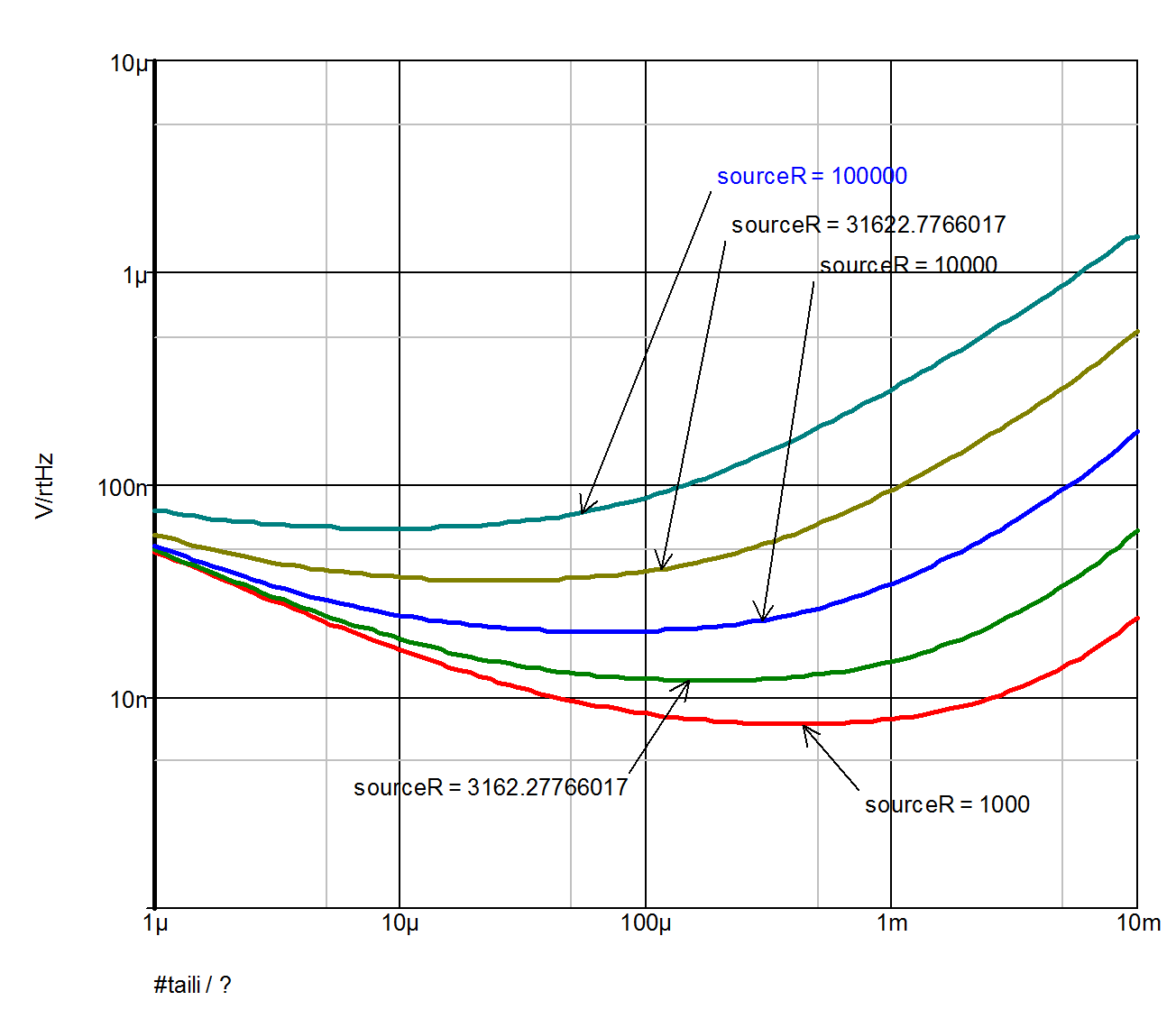
Refer to circuit in Plotting Results of Noise Analysis, Example 2. In the previous example we swept the tail current to find the optimum value to minimise noise for a 1K source resistance. Here we extend the example further so that the run is repeated for a range of source resistances. The source resistance is varied by performing a parameter step on sourceR. Here is what the dialog settings are for the multi-step run:

This does a decade sweep varying sourceR from 1K to 100k with 2 steps per decade. This is the result we get:
Example 2
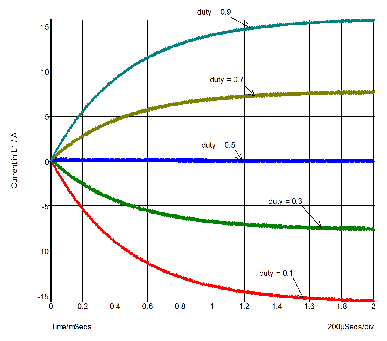
The following circuit is a simple model of a full bridge switching amplifier used to deliver a controlled current into an inductance.
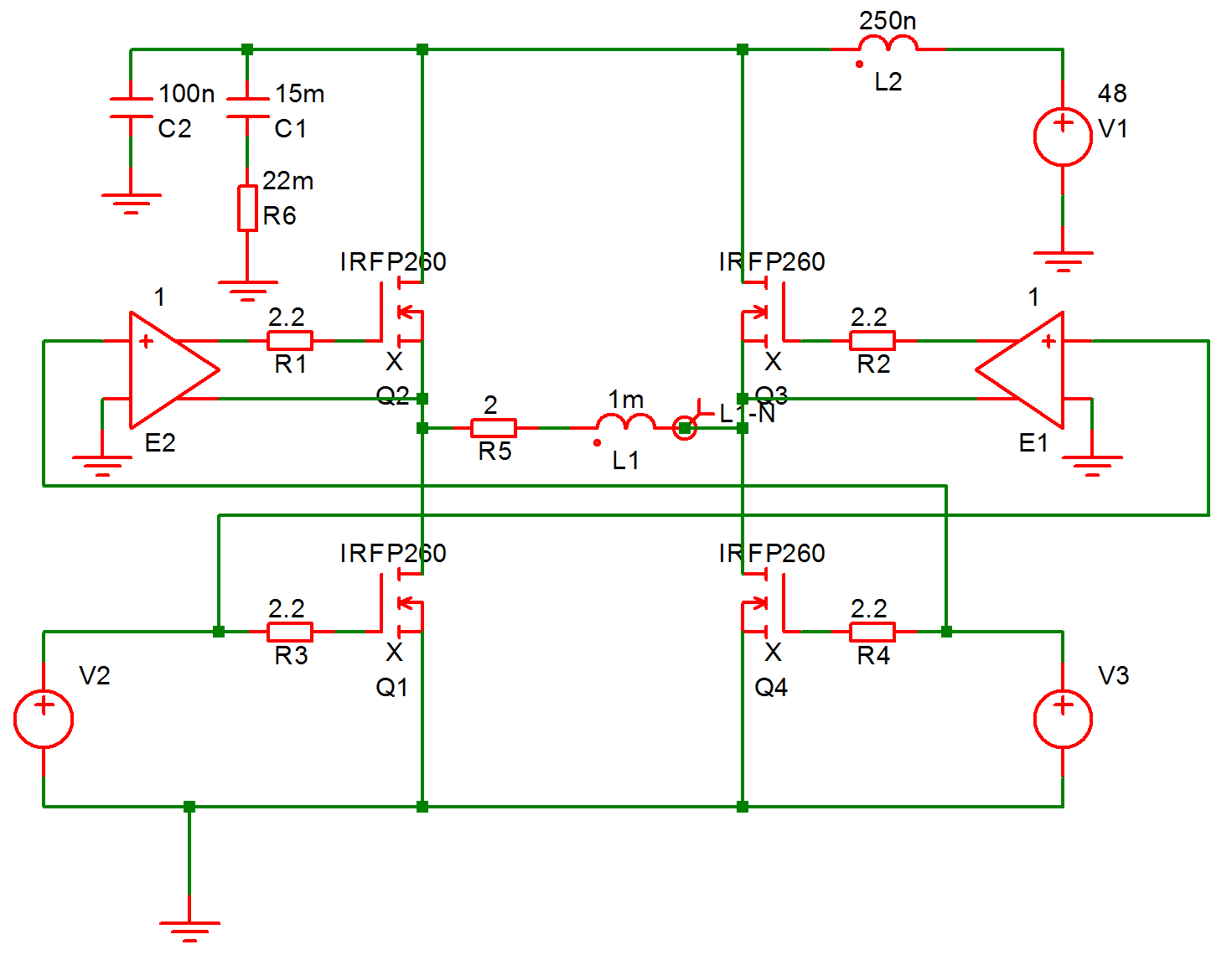
Sources V2 and V3 have been defined to be dependent on a parameter named duty which specifies the duty cycle of the switching waveform. See EXAMPLES/BRIDGE/BRIDGE.sxsch.
This was setup to perform a multi step analysis with the parameter duty
stepped from 0.1 to 0.9. This is the result:
| ◄ Simulator Options | Safe Operating Area Testing ▶ |