Fixed Probes
There are many types of fixed probe as described in the following table
| Probe Type | Description | To Place |
| Voltage | Single ended voltage. Hint: If you place the probe immediately on an existing schematic wire, it will automatically be given a meaningful name related to what it is connected to | Menu: Hot key: B |
| Current | Device pin current. A single terminal device to place over a device pin | Menu: Hot key: U |
| Inline current | In line current. This is a two terminal device that probes the current flowing through it. | Menu: |
| Differential voltage | Probe voltage between two points | Menu: |
| dB | Probes db value of signal voltage. Only useful in AC analysis | Menu: |
| Phase | Probes phase of signal voltage. Only useful in AC analysis | Menu: |
| Bode plot with Measurements | Plots db and phase of vout/vin. Connect to the input and output of a circuit to plot its gain and phase. Includes optionsl measurements for phas margin, gain margin and gain crossover frequency | Menu: |
| Bode plot - basic version | Plots db and phase of vout/vin. Connect to the input and output of a circuit to plot its gain and phase. | Menu: |
| Bus plot | Plots bus signal in 'logic analyser' style | Menu: |
| Power plot | Plots the power in a device. The power probe must be attached to a single pin of the device. It doesn't matter which pin - the power plotted in the instantaneous power in the whole device | Menu: |
| Per Cycle | Plot a graph based on a calculation performed for each complete cycle of a repetitive waveform. See Per Cycle Probes | Available from Parts Selector |
| X-Y | Plot a graph of one signal on the y-axis with respect to a second signal on the x-axis. See X-Y Probes | Menu: |
Current probes and power probes must be placed directly over a part pin. They will have no function if they are not and a warning message will be displayed.
In this topic:
Fixed Probe Options
All probe types have a large number of options allowing you to customise how you want the graph plotted. For many applications the default settings are satisfactory. In this section, the full details of available probe options are described. Select the probe and press F7 or menu Edit Part...
The following dialog will be displayed for voltage, current, power, db and phase probes:
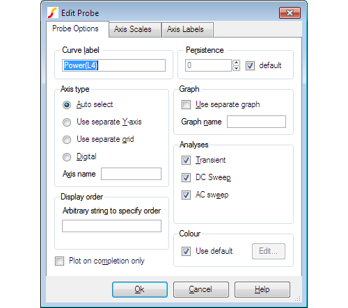
The elements of each tabbed sheet are explained below.
Probe Options Sheet
| Curve Label | Text displayed by the probe on the schematic and also used to label the resulting curves | ||||||||
| Persistence |
The number of curves from a single probe that will be displayed at once.
|
||||||||
| Axis type |
Specifies the type of y-axis to use for the curve.
|
||||||||
| Graph | Check Use Separate Graph to create a new graph sheet for the probe. You may also supply a graph name, which works the same way as axis name described above. this is not a label but a means of identification. Any other probes using the same graph name will have their curves directed to the same graph sheet. | ||||||||
| Analyses | Specifies for which analyses the probe is enabled. Note: Other analysis modes such as noise and sensitivity are not included because these do not support schematic cross probing of current or voltage. For SIMPLIS mode, a Periodic Operating Point (POP) option is also available. | ||||||||
| Display order | Enter a string to control the grid display order. The value is arbitrary and will not be displayed. To force the curve to be placed above other curves that don't use this value, prefix the name with '!'. The '!' character has a low ASCII value. Conversely, use '~' to force curve to be displayed after other curves. | ||||||||
| Colour | Check Use default to minimise duplicate colours on the same graph by allowing the colour to be chosen automatically. Alternatively uncheck, this box and then press Edit... to select a colour of your choice. In this case the trace always has the same colour. | ||||||||
| Plot on completion only |
|
Axis Scales Sheet
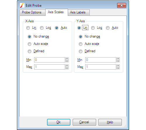
| Parameter | Description |
| Lin/Log/Auto |
Specify whether you want X-Axis to be linear or logarithmic.
|
| No Change Auto scale Defined |
Controls how the axis limits are defined
|
Axis Labels Sheet
This sheet has four edit boxes allowing you to specify, x and y axis labels as well as their units. If any box is left blank, a default value will be used or will remain unchanged if the axis already has a defined label.
Fixed Bus Probe Options
Select device and press F7 in the usual manner. A dialog box will show similar to that shown in Bus Probe Options. But you will notice an additional tabbed sheet titled Probe Options. This allows you to select an axis type and graph in a similar manner to that described above for fixed voltage and current probes.
Using Fixed Probes in Hierarchical Designs
Fixed probes may successfully be used in hierarchical designs. If placed in a child schematic, a plot will be produced for all instances of that child and the labels for each curve will be prefixed with the child reference.
Adding Fixed Probes After a Run has Started
When you add a fixed single ended voltage or current probe after a run has started, the graph of the probed point opens soon after resuming the simulation. To do this:
- Pause simulation.
- Place a probe on the circuit in the normal way.
- Resume simulation
Per-cycle Probes
- Single-ended voltage
- Differential voltage
- Current
- Difference of two currents
| Per-cycle Probes | |
| Model Name: | Per Cycle Probes |
| Simulator: | The device is compatible with the SIMetrix and SIMPLIS simulators |
| SIMetrix Parts Selector Location: | |
| SIMPLIS Parts Selector Location: | |
| Symbol Library: | None the symbol is automatically generated when placed |
| Symbols: |
|
| Multiple Selections: | Multiple probes can be selected and edited simultaneously. |
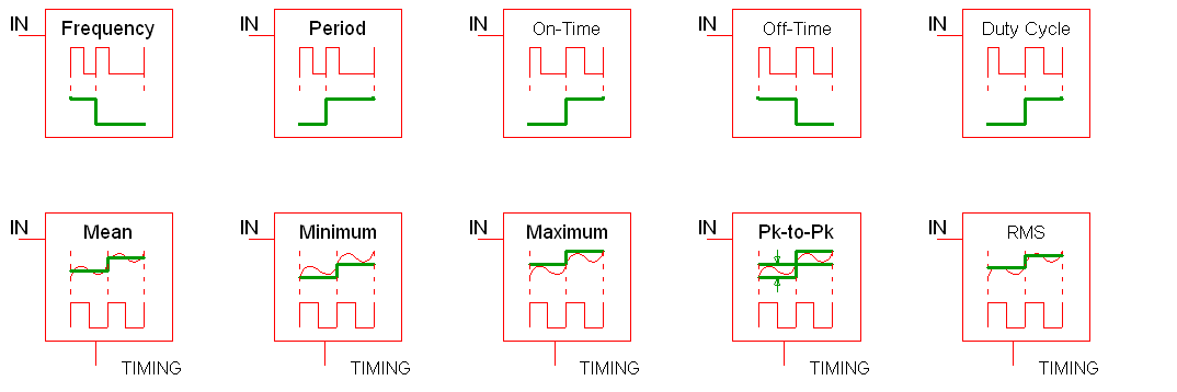
Per-Cycle Timing Measurements
 The following timing measurements are supported on a per-cycle basis:
- Frequency
- Period
- Duty Cycle
- On Time
- Off Time
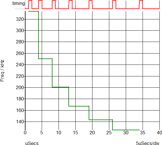
Per-Cycle Amplitude Measurements
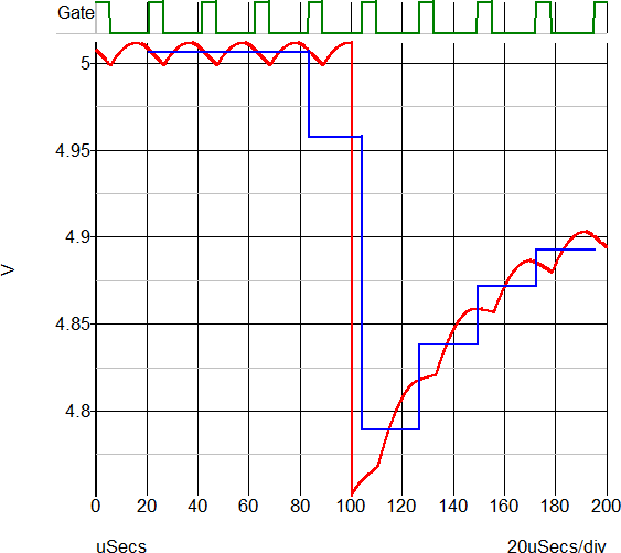
The per-cycle measurement can also be applied to amplitude of an input voltage or current. For example, you can plot the mean value of a switching power converter output with the mean value being calculated on a per-cycle basis. This example is show below - the mean value of a converter output voltage is plotted in a per-cycle manner. The gate voltage is used to determine the timing edge information.
 The following amplitude measurements are supported:
- Mean
- Maximum
- Minimum
- RMS
- Peak to Peak
Editing the Per Cycle Probe
- Double click the symbol on the schematic to open the editing dialog to the Probe Options tab.
- Make the appropriate changes on the three tabs as explained below.
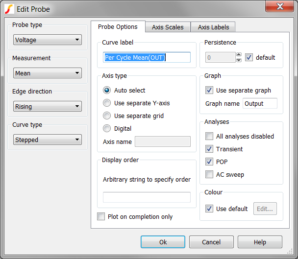
Per Cycle Probe Options
The following tab allows you to define general probe options, which are explained in the table below.
| Parameter | Description | ||||||||
| Measurement | Frequency, Period, On-Time, Off-Time, Duty Cycle, Mean Maximum, Minimum, Peak-to-Peak, or RMS | ||||||||
| Edge Direction | Rising, Falling or Both | ||||||||
| Curve type | Stepped or Smooth | ||||||||
| Curve Label | Text displayed by the probe on the schematic and also used to label the resulting curves | ||||||||
| Persistence |
The number of curves from a single probe that will be displayed at once.
|
||||||||
| Axis type |
Specifies the type of y-axis to use for the curve.
|
||||||||
| Graph | Check Use Separate Graph to create a new graph sheet for the probe. You may also supply a graph name, which works the same way as axis name described above. this is not a label but a means of identification. Any other probes using the same graph name will have their curves directed to the same graph sheet. | ||||||||
| Analyses | Specifies for which analyses the probe is enabled. Note: Other analysis modes such as noise and sensitivity are not included because these do not support schematic cross probing of current or voltage. For SIMPLIS mode, a Periodic Operating Point (POP) option is also available. | ||||||||
| Display order | Enter a string to control the grid display order. The value is arbitrary and will not be displayed. To force the curve to be placed above other curves that don’t use this value, prefix the name with '!'. The '!' character has a low ASCII value. Conversely, use '~' to force curve to be displayed after other curves. | ||||||||
| Colour | Check Use default to minimise duplicate colours on the same graph by allowing the colour to be chosen automatically. Alternatively uncheck, this box and then press Edit... to select a colour of your choice. In this case the trace always has the same colour. | ||||||||
| Plot on completion only | This option is not available with per-cycle probes and the setting of the check box will be ignored. |
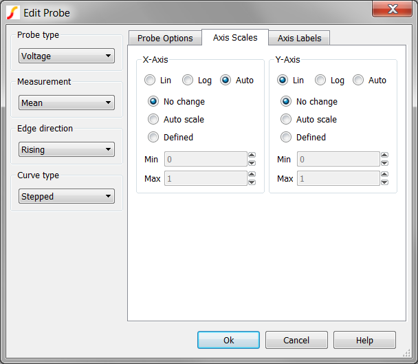
Axis Scales
The following tab allows you to define the scale for the X-axis and for the Y-axis as explained in the table below.
| Parameter | Description |
| Lin/Log/Auto |
Specify whether you want X-Axis to be linear or logarithmic.
|
| No Change Auto scale Defined |
Controls how the axis limits are defined
|
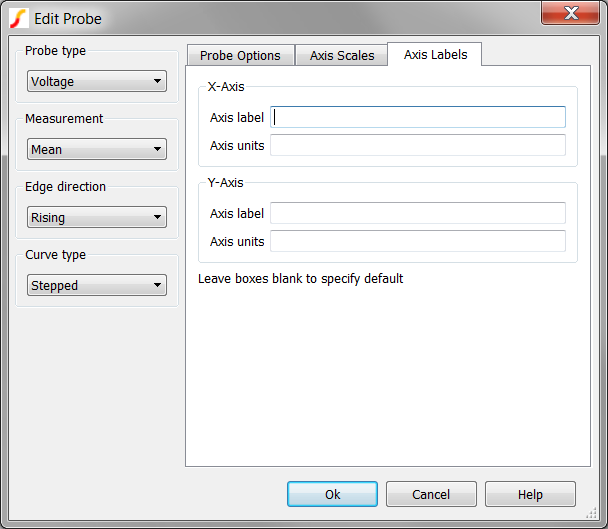
Axis Labels
To specify axis labels and units, click the Axis Labels tab, and enter values as needed.
Note: If any box is left blank, a default value is used or remains unchanged if the axis already has a defined label.
XY Probes
| XY Probes | |
| Model Name: | XY Probe |
| Simulator: | This device is compatible with the SIMetrix and SIMPLIS simulators. |
| Part Selector Location: | |
| Symbol Library: | connection.sxslb |
| Symbols: |
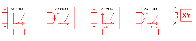
|
| Multiple Selections: | Multiple probes can be selected and edited simultaneously. |
Editing the XY Probe
- Double click the symbol on the schematic to open the editing dialog to the Probe Options tab.
- Make the appropriate changes on the three tabs as explained below.
XY Probe Options
The following tab allows you to define general probe options, which are explained in the table below.
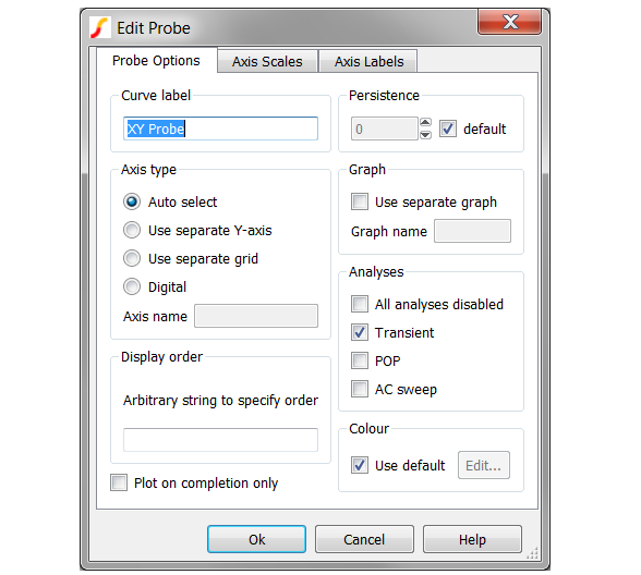
| Curve Label | Text displayed by the probe on the schematic and also used to label the resulting curves | ||||||||
| Persistence |
The number of curves from a single probe that will be displayed at once.
|
||||||||
| Axis type |
Specifies the type of y-axis to use for the curve.
|
||||||||
| Graph | Check Use Separate Graph to create a new graph sheet for the probe. You may also supply a graph name, which works the same way as axis name described above. this is not a label but a means of identification. Any other probes using the same graph name will have their curves directed to the same graph sheet. | ||||||||
| Analyses | Specifies for which analyses the probe is enabled. Note: Other analysis modes such as noise and sensitivity are not included because these do not support schematic cross probing of current or voltage. For SIMPLIS mode, a Periodic Operating Point (POP) option is also available. | ||||||||
| Display order | Enter a string to control the grid display order. The value is arbitrary and will not be displayed. To force the curve to be placed above other curves that don’t use this value, prefix the name with '!'. The '!' character has a low ASCII value. Conversely, use '~' to force curve to be displayed after other curves. | ||||||||
| Colour | Check Use default to minimise duplicate colours on the same graph by allowing the colour to be chosen automatically. Alternatively uncheck, this box and then press Edit... to select a colour of your choice. In this case the trace always has the same colour. | ||||||||
| Plot on completion only | This option is not available with XY Probes and the check box setting will be ignored. |
Axis Scales
| Parameter | Description |
| Lin/Log/Auto |
Specify whether you want X-Axis to be linear or logarithmic.
|
| No Change Auto scale Defined |
Controls how the axis limits are defined
|
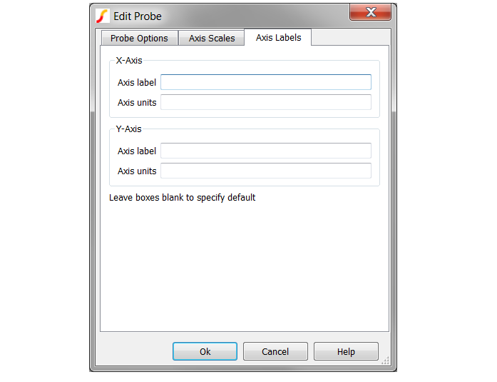
Axis Labels
To specify axis labels and units, click the Axis Labels tab, and enter values as needed.
Note: If any box is left blank, a default value is used or remains unchanged if the axis already has a defined label.
Bode Plot Probe with Measurements
The Bode Plot Probe with Measurements generates plots for the gain and phase of the ratio of two voltages. The probe can be configured to plot only the gain or phase, or both gain and phase.
| Summary - Bode Plot Probe with Measurements | |
| Model Name | Bode Plot Probe |
| Simulator | This device is compatible with both SIMetrix and SIMPLIS simulators |
| Schematic Menu | |
| Parts Selector | |
| Symbol Library | Connections |
| Model File | none |
| Symbol |

|
| Multiple Selections | If multiple Bode plot probes are selected before editing, all properties except the curve labels can be simultaneously changed for all probes. The curve label properties will remain unchanged for all selected probes |
| Usage | This schematic probe symbol plots the magnitude and phase of the ratio of two complex voltages, OUT/IN. The magnitude can be plotted in db or volts/volts; the horizontal axis scale is determined by the simulation sweep type. If the simulation is swept in log frequency steps, the horizontal axis will automatically be log scaled |
Editing the Bode Plot Probe with Measurements
- Double click the symbol on the schematic to open the editing dialog to the Parameters tab.
- Make the appropriate changes to the fields described in the table below the image.
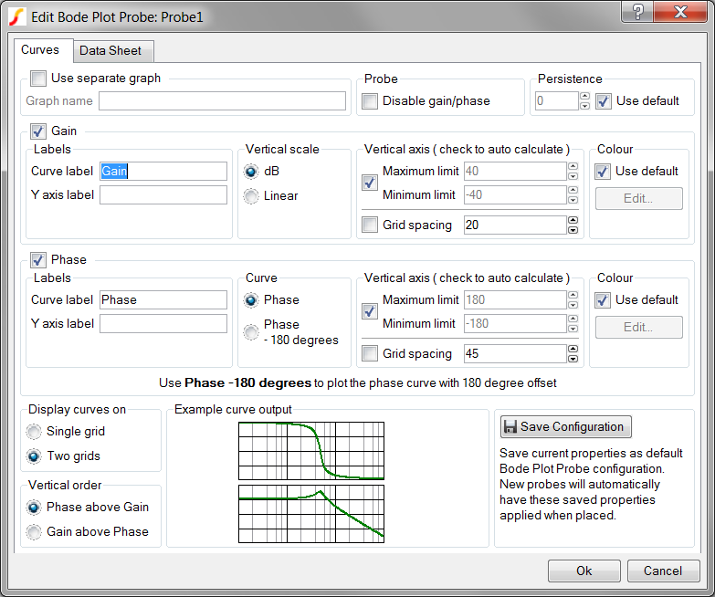
| Options - Bode Plot Probe with Measurements | |
| Use separate graph | Check this option in order to supply an alias for each output graph tab |
| Graph name | The Graph name is an alias for each output graph tab and will not be visible on the graph output. Curves with the same graph name property will be output on the same graph tab. Graph name be safely ignored unless multiple Bode plot probes are used. Use separate graph must be checked to supply this name. |
| Disable gain/phase | Check this box to disable both gain and phase graphs |
| Persistence |
The Persistence property determines when previous simulation data is deleted from the graph viewer. If Use default is checked or if the persistence is set to -1, the probe uses the default global persistence value.
The default persistence can be set from the command shell menu:
|
| Curve label | Sets the name of the curve. Note: This field appears in both the Gain and Phase groups on the dialog |
| Y axis label | Sets the Y axis label for the individual gain and phase axes. When multiple curves from multiple probes are placed on the same axis, the axis label properties must be identical or the axis label is blank. If this field is left blank, the axis label appears with the name specified in the Curve label field. Note: This field appears in both the Gain and Phase groups on the dialog |
| Vertical scale |
Allows you to select the function to perform on the simulation data.
|
| Curve |
Selects the Phase curve offset
|
| Vertical axis |
This group has two options:
Vertical limits
|
| Colour |
Defines colours for the curves:
|
| Display curves on | Allows you to define the number of grids in the output: Single grid or Two grids |
| Vertical order |
Allows you to specify the order of the curves: Phase above Gain or Gain above Phase.
|
| Example curve output | Example curve output illustrates the relative locations of the two curves. Note: The curve data here is fixed; these curves are examples and do not reflect the simulated curves |
| Save Configuration | Click Save Configuration to preserve this information as the default configuration for all future new Bode plot probes |
Bode Plot Probe - Basic Version
Connects to the input and output of a circuit to plot its gain and phase. A more sophisticated bode plot probe which provides a wide range of options along with the display of useful measurements is also available and is recommended for most applications. See Bode Plot Probe with Measurements
This basic version is useful for quick checks and for compatibility with versions 7.0 or earlier.
| Summary - Bode Plot Probe - Basic | |
| Model Name | Bode Plot Probe - Basic |
| Simulator | This device is compatible with both SIMetrix and SIMPLIS simulators |
| Schematic Menu | |
| Parts Selector | |
| Symbol Library | Connections |
| Model File | none |
| Symbol |

|
| Multiple Selections | If multiple Bode plot probes are selected before editing, all properties except the curve labels can be simultaneously changed for all probes. The curve label properties will remain unchanged for all selected probes |
| Usage | This schematic probe symbol plots the magnitude and phase of the ratio of two complex voltages, OUT/IN. The magnitude can be plotted in db or volts/volts; the horizontal axis scale is determined by the simulation sweep type. If the simulation is swept in log frequency steps, the horizontal axis will automatically be log scaled |
Editing Bode Plot Probe
- Double click the symbol on the schematic to open the editing dialog to the Parameters tab.
- Make the appropriate changes to the fields described in the table below the image.
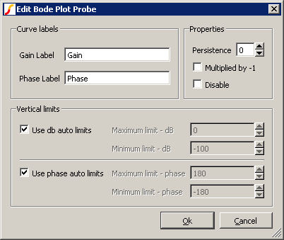
| Options - Bode Plot Probe | |
| Curve labels |
Sets labels for plots
|
| Properties |
Set additional properties on probe:
|
| Vertical Limits |
Divided into two parts to allow setting of axis limits for phase and gain plots.
|
Fourier Analysis
A fixed Fourier probe is available which will perform a spectral analysis on a node voltage. To place this probe, select menu .
Double click the probe to edit it. You will see this dialog box:
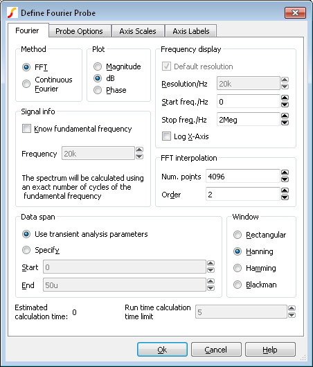
The settings are similar to that for random Fourier probe plotting as described here: Fourier Analysis. The documentation is repeated here for convenience.
Method
SIMetrix offers two alternative methods to calculate the Fourier spectrum: FFT and Continuous Fourier.
The simple rule is: use FFT unless the signal being examined has very large high frequency components as would be the case for narrow sharp pulses.
A description of the two techniques and their pros and cons follows.
| FFT | Fast Fourier Transform. This is an efficient algorithm for calculating a discrete Fourier transform or DFT. DFTs generally operate on evenly spaced sampled data. Unfortunately the data generated by the simulator is not evenly spaced so it is therefore necessary to interpolate the data before presenting it to an FFT algorithm. The interpolation process is in effect the sampling process and the Nyquist sampling theorem applies. This states that the signal can be perfectly reproduced from the sampled data if the sampling rate is greater than twice the maximum frequency component in the signal. In practice this condition can never be met perfectly and any signal components whose frequency is greater than half the sampling rate will be aliased to a different frequency. So if the number of interpolated points is too small there will be errors in the result due to high frequency components being aliased to lower frequencies. This is the Achilles heel of FFTs applied to simulated data. The Continuous Fourier technique, described next, does not suffer from this problem. It suffers from other problems the main one being that it is considerably slower than the FFT. |
| Continuous Fourier | This calculates the Fourier spectrum by numerically integrating the Fourier integral. With this method, each frequency component is calculated individually whereas with the FFT the whole spectrum is calculated in one - quite efficient - operation. Continuous Fourier does not require the data to be interpolated and does not suffer from aliasing. The problem with continuous Fourier is that compared to the FFT it is a slow algorithm and in many cases an FFT with a very large number of interpolated points can be calculated more quickly and give just as accurate a result. However, in cases where a signal has a very large high frequency content - such as narrow pulses - this method is superior and it is recommended that it is used in preference to the FFT in such situations. The continuous Fourier technique has the additional advantage that it can be applied with greater confidence as the aliasing errors will not be present. It does have its own source of error due to the fact that simulated data itself is not truly continuous but represented by unevenly spaced points with no information about what lies between the points. This error can be minimised by ensuring that close simulation tolerances are used. See Simulator Reference Manual/Convergence, Accuracy and Performance for details. |
Plot (Phase or Magnitude)
The default is to plot the magnitude of the Fourier spectrum. Select Phase if you require a plot of phase or dB if you need the magnitude in dBs.
Frequency Display
| Resolution/Hz | Available only for the continuous Fourier method. This is the frequency interval at which the spectral components are evaluated. It cannot be less than 1/T where T is the time interval over which the spectrum is calculated. |
| Start Freq./Hz | Start frequency of the display. |
| Stop Freq./Hz | Stop frequency of the display. |
| Log X-Axis | Check this to specify a logarithmic x-axis. This will force a minimum value for the start frequency equal to 1/T where T is the time interval being analysed. |
Signal Info
If the signal being analysed is repetitive and the frequency of that signal is known exactly then a much better result can be obtained if it is specified here. Check the Know fundamental frequency box then enter the frequency. The Fourier spectrum will be calculated using an integral number of complete cycles of the fundamental frequency. This substantially reduces spectral leakage. Spectral leakage occurs because both the Fourier algorithms work on an assumption that the signal being analysed is a repetition of the analysed time interval from ???MATH???t=-\infty???MATH??? to ???MATH???t=+\infty???MATH???. If the analysed time interval does not contain a whole number of cycles of the fundamental frequency this will be a poor approximation and the spectrum will be in error. In practice this problem is minimised by using a window function applied to the signal prior to the Fourier calculation, but using a whole number of cycles reduces the problem further.
Note that the fundamental frequency is not necessarily the lowest frequency in the circuit but the largest frequency for which all frequencies in the circuit are integral harmonics. For example if you had two sine wave generators of 1kHz and 1.1KHz, the fundamental is 100Hz, not 1kHz; 1kHz is the tenth harmonic, 1.1KHz is the eleventh.
You should not specify a fundamental frequency for circuits that have self-oscillating elements.
FFT Interpolation
As explained above, the FFT method must interpolate the signal prior to the FFT computation. Specify here the number of points and the order. The number of points entry may be forced to a minimum if a high stop frequency is specified in the Frequency Display section.
The number of interpolation points required depends on the highest significant frequency component in the signal being analysed. If you have an idea what this is, a useful trick to set the number of points to a suitable value, is to increase the stop frequency value in the Frequency Display section up to that frequency. This will automatically set the number of interpolation points to the required value to handle that frequency. If you don't actually want to display frequencies up to that level, you can bring the stop frequency back down again. The number of interpolation points will stay at the value reached.
If in doubt, plot the FFT twice using a different number of points. If the two results are significantly different in the frequency band of interest, then you should increase the number of points further.
Usually an interpolation order of 2 is a suitable value but you should reduce this to 1 if analysing signals with abrupt edges. If analysing a smooth signal such as a sinusoid, useful improvements can be gained by increasing the order to 3.
Data Span
Usually the entire simulated time span is used for the Fourier analysis. To specify a smaller time interval click Specify and enter the start and end times.
Note that if you specify a fundamental frequency, the time may be modified so that a whole number of cycles is used. This will occur whether or not you explicitly specify an interval.
Window
A window function is applied to the time domain signal to minimise spectral leakage (See above).
The choice of window is a compromise. The trade off is between the bandwidth of the main spectral component or lobe and the amplitude of the side-lobes. The rectangular window - which is in effect no window - has the narrowest main lobe but substantial side-lobes. The Blackman window has the widest main lobe and the smallest side lobes. Hanning and Hamming are something in between and have similar main lobe widths but the side lobes differ in the way they fall away further from the main lobe. Hamming starts smaller but doesn't decay whereas Hanning while starting off larger than Hamming, decays as the frequency moves away from the central lobe.
Despite the great deal of research that has been completed on window functions, for many applications the difference between Hanning, Hamming and Blackman is not important and usually Hanning is a good compromise.
There are situations where a rectangular window can give significantly superior results. This requires that the fundamental frequency is specified and also that the simulated signal is consistent over a large number of cycles. The rectangular window, however, usually gives considerably poorer results and must be used with caution.
Run time calculation time limit
If using the Continuous Fourier method, you can enter a maximum time limit to calculate the Fourier spectrum. If the limit is exceeded, the calculation will abort and no display will be made. The Continuous Fourier calculation time can be excessive but cannot be predicted before the simulation is started as it is necessary to know the number of simulation time points to be processed.
For the FFT method, the simulation time can be estimated to a reasonable accuracy before the simulation and this estimate will be displayed labelled Estimated calculation time:.
Custom Fixed Probe
You can create an arbitrary fixed probe to plot an expression of any combination of node voltages and device currents. To use this feature, select menu . You will see this dialog box:
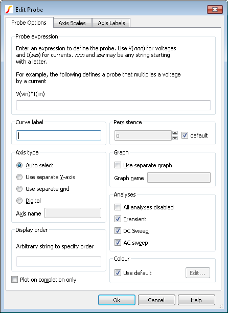
Probe expression
Enter an expression to define what you wish to be plotted. Use V(nnn) to access a voltage and I(sss) to access a current. nnn and sss may be any arbitrary string starting with a letter. When you close the dialog box a symbol will be created which will reflect what you enter here. It will have single inputs named according to occurrences of V(nnn) and pairs of inputs named after occurrences of I(sss). For example if you enter the expression:
V(vin)*I(iin)
The symbol created will look like this:
\begin{figure}[H] \centering \includegraphics[width=0.4\linewidth]{images/Custom-probe-symbol.png} \end{figure}
The result plotted will be the product of the voltage on vin and the current in iin.
The same behaviour could be achieved using a Non-linear transfer function device (see Non-linear Transfer Function ) and a simple single ended probe. This arbitrary probe has some important advantages over that approach:
- The arbitrary probe works in SIMPLIS simulations. The Non-linear transfer function device is a SIMetrix-only device.
- It can evaluate non-linear functions in AC analysis
- It is a post-processing operation and does not interfere with the simulation in any way
Other Arbitrary Probe Options
The other options are the same as for standard fixed probes. Refer to Fixed Probe Options
Changing Update Period and Start Delay
The update period of all fixed probes can be changed from the Options dialog box. Select menu and click on the Graph/Probe/Data analysis tab. In the Probe update times/seconds box there are two values that can be edited. Period is the update period and Start is the delay after the simulation begins before the curves are first created.
| ◄ Probes: Fixed vs. Random | Random Probes ▶ |