3.1 SIMPLIS Multi-Step Analysis
The ability to step or sweep parameters enables quick design verification. In this topic, you will setup and sweep the RLoad parameter and then learn how to nest a sweep of the input voltage with the output load. In this multi-step simulation you will verify the converter performance over both the input voltage range and the output load range.
To download the examples for Module 3, click Module_3_Examples.zip
In this topic:
Key Concepts
This topic addresses the following key concepts:
- Design parameters can be swept with a linear or decade sweep, or over a range of values.
- Multiple parameters can be stepped in nested sweeps by hand-editing the multi-step configuration file.
- Multiple processor cores can be used to reduce the time required to execute a Multi-Step simulation.
- Multiple curves can be grouped into a single curve by either selecting the Group curves check box or by editing the groupCurves= entry in the configuration file.
What You Will Learn
In this topic, you will learn the following:
- How a parameter can be stepped through a list of values, with one simulation executed per value.
- How parameters can swept over a range of values using a linear or decade sweep to determine the step size.
- How to setup and run multi-step simulations.
- How to use multiple processor cores to reduce the time required to execute a Multi-Step simulation.
Getting Started
- Close the waveform viewer if it is open.
- Open the schematic 3.1_SelfOscillatingConverter_POP.sxsch.
- From the schematic menu, select .Result: The Define SIMPLIS Multi-Step Analysis dialog opens:
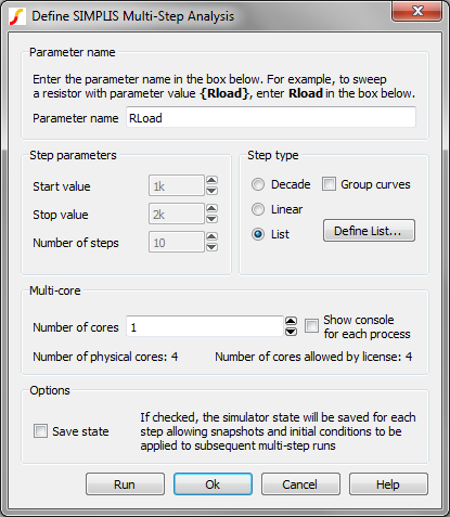
- The dialog is already prepared to step the parameter RLoad through a list of
values. To view the list of values, click on the Define List... button.Result: The Define List dialog opens, displaying the three RLoad step values: 5,2.5, and 4.2.
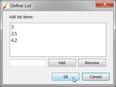
- Click Ok on the Define List dialog.
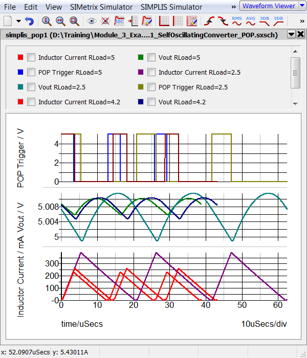
- Click Run on the Define SIMPLIS Multi-Step Analysis dialog.Result: The Multi-Step simulation runs and the periodic operating point waveforms for each RLoad value are displayed on the waveform viewer: Note that the converter switching frequency, peak inductor current, and output ripple changes for each simulated RLoad value.
Discussion
The SIMPLIS Multi-Step Analysis allows you to quickly verify how a design responds to parameter changes. In the next topic, 3.2 Monte-Carlo Simulations, you will learn how the SIMPLIS Monte-Carlo Analysis allows you to vary multiple design parameters with statistical distributions.
In this example, three RLoad values which couldn't be defined as a linear or decade sweep were chosen. The List sweep option allows you to choose any list of values. The SIMPLIS Multi-Step Analysis allows you to sweep parameters over linear or decade steps as well. More information on the different sweep types can be found in the help topic linked to by the Help button on the Define SIMPLIS Multi-Step Analysis dialog.
How The Multi-Step Analysis Works
You may recall from the topic 3.0.1 What Happens When You Press F9? that the RLoad variable is set in the F11 window:
.var RLoad=2.5
When you ran the Multi-Step Analysis, the RLoad value defined in the F11 window was overwritten by the step value defined in the Define SIMPLIS Multi-Step Analysis dialog. For each step value, the netlist preprocessor:
- Includes the stepped parameter value, in this case RLoad.
- Pre-processes the netlist
- Launches the SIMPLIS simulator on the resulting deck.
In this example, three individual deck files were created, and each new deck file over-writes the previous deck file. This example steps the RLoad parameter over three values in the order - 5 , 2.5, 4.2. In the last deck file, R3 will have a value of 4.2Ω. In the next exercise you will verify the last value of R3 is 4.2Ω.
Exercise #1: Verify R3 Value
- From the menu bar, select .Result: The Deck file opens in the netlist editor.
- To search for the text 4.2, follow these steps:
- Use the shortcut key Ctrl+F to open the search dialog.
- Type 4.2Result: the deck file scrolls to line 108 where the value of R3 is 4.2 Ω.
107 R2 35 0 1.5 108 R3 41 0 4.2 109 R2 0 28 150
SIMPLIS Multi-Core Capability
The SIMetrix/SIMPLIS Pro and Elite licenses can use multiple processor cores to simulate the stepped parameter values. Using multiple cores allows multiple step values to be simultaneously simulated. The number of cores allowed by the licenses are:
| License | Number of Physical Cores |
| Pro | 4 |
| Elite | 16 |
In addition to the maximum number of cores allowed by your license, you are obviously limited by the number of cores your computer has. For this limitation, SIMetrix/SIMPLIS only uses the physical cores, not the hyper-threaded cores. In the next exercise you will run a multi-core, multi-step simulation.
Exercise #2: Enable Multi-Core
This exercise assumes your computer has more than one physical core and that you are using a SIMetrix/SIMPLIS Pro license.
- Close the waveform viewer.
- From the schematic menu, select .Result: The Define SIMPLIS Multi-Step Analysis dialog opens:
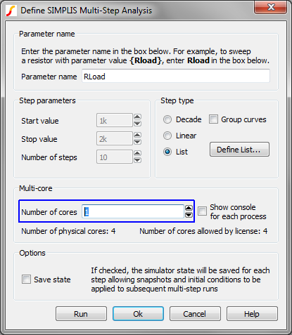
- Change the Number of cores to 4, the maximum allowed by the Pro license.
Note: If your machine has either a single core or two cores, the dialog will limit your Number of cores entry. If you have a single core, you can skip this exercise.
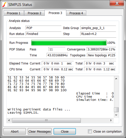
- Click Run.Result: The Multi-Step simulation runs on the maximum number of physical cores. Assuming you have a 4 Core machine, all 3 step values are executed simultaneously using 3 SIMPLIS processes, one per processor core. The SIMPLIS Status window has four tabs, one for each SIMPLIS process. The fourth tab is empty as no step value was run on this process:
In this exercise, a very small circuit was simulated, yet you probably noticed a significant speed improvement in the time required to execute the Multi-Step Analysis. As circuit size grows, this effect becomes dramatic, and in experiments, speed improvements of approximately 3.5 times when using 4 cores vs. a single core have been found.
Stepping Multiple Parameters in the Multi-Step Analysis
The information entered in the Define SIMPLIS Multi-Step Analysis dialog is written to a Multi-Step Configuration file. This file is saved in the same directory as the schematic and has the same name as the schematic except the file extension is ".sxscf." Although the editing dialog allows one parameter to be stepped over a range of values, by hand editing the Multi-Step Configuration file in a text editor, you can step multiple parameters each over its own range of values.
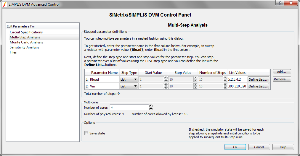
In this exercise, in addition to stepping the load resistor over a range of three values, you will also step the converter input voltage over a range of three values. Because the steps are nested, a total of 9 simulation steps will be executed. In other words, for each value of RLoad the input voltage will be varied over each of value of its parameter range. This test verifies the converter operation over the minimum, typical, and maximum values of both the input voltage and output load.
Exercise #3: Stepping Multiple Parameters in the Multi-Step Analysis
- Right click on the gray bar at the top of the schematic:
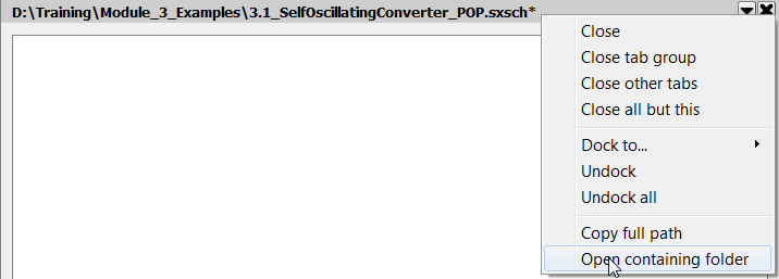 Result: The context menu appears with options for this window.
 - Select the Open Containing Folder menu option.Result: a Windows Explorer window opens to the schematic directory.
- Select the 3.1_SelfOscillatingConverter_POP.sxscf file, and drag it into
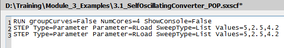
the SIMetrix/SIMPLIS Main Window.Result: The file opens in the netlist editor. This file contains the commands which the program interprets when executing a Multi-Step Analysis. The second line has the RLoad parameter information.
- To step the Vin parameter, you will copy the second line and enter the
copied line on the third line of this file, following these steps:
- Select all the text on line 2.
- Copy to the windows clipboard with the keyboard shortcut Ctrl+C.
- Move the cursor to line 3.
- Paste the data using the keyboard shortcut Ctrl+V.Result: The text file now has three lines. Line 3 is a duplicate of line 2.
- To edit Line #3:
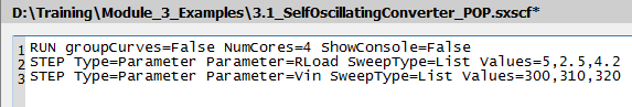
- Change RLoad to Vin.
- Change the values at the end of the line from 5,2.5,4.2 to
300,310,320.Result: The final text file should appear exactly as follows:
- Save the file using the keyboard shortcut Ctrl+S.
- Close the waveform viewer.
- In SIMetrix/SIMPLIS, run the Multi-Step Analysis with the menu .Result: The Multi-Step Analysis executes and curves for the 9 step value combinations are output to the waveform viewer. As three probes are enabled, 27 curves are output to the waveform viewer.
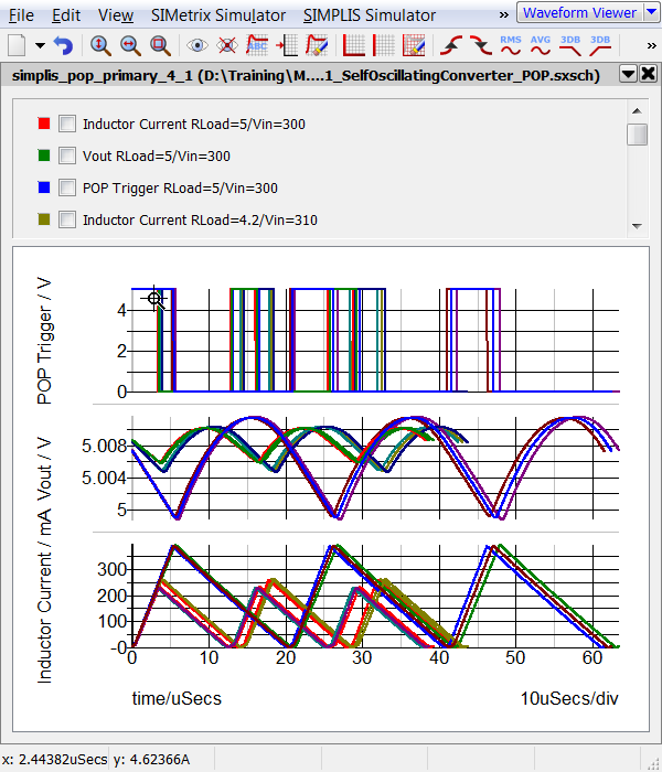
Discussion: Exercise #3
As you can see, multi-step analyses with multiple parameters increases the number of simulation runs geometrically. You can easily fill up the waveform viewer legend with curve information to the point where it is hardly navigable. You can reduce the cluttered graph legend by telling the program to "Group" the curves that each probe outputs into a single curve with a single color. In the next exercise you will edit the Multi-Step Configuration file to group the output curves into a single curve for each probe.
Exercise #4: Group Output Curves
- In the text editor window, find the groupCurves=False text on the first
line:
- Change the groupCurves=False text to groupCurves=True. The final
file will appear exactly as follows:

- Save the file using the keyboard shortcut Ctrl+S.Result: the disk icon turns from red to light blue indicating the file has been saved.
- Close the waveform viewer.
- In SIMetrix/SIMPLIS, run the Multi-Step Analysis with the menu .Result: The Multi-Step Analysis executes as before, but three curves are output, each curve has nine traces representing the nine stepped values.
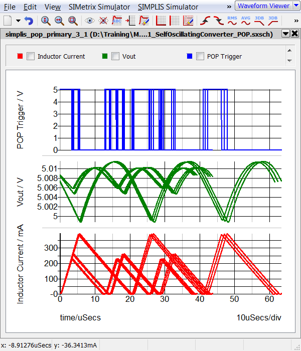
Discussion: Exercise #4
Each curve listed in the graph legend depicts data generated by the 9 steps of Multi-Step data. The nine steps use the same color and a single entry in the graph legend. A few points should be made:
- The grouped data presented in the graph above is written to a Multi-Division data group. Analysis of Multi-Division data is extremely challenging, and has to be performed using custom scripts via the SIMetrix/SIMPLIS script language. The built-in measurement system used by the waveform viewer was not designed to handle Multi-Division data.
- The Design Verification Module, which was specifically designed to analyze and present data from multiple single-step simulations in which more than one parameter is stepped, outputs multiple single step data files, one for each combination of parameter values. The analysis of this data is both trivial, and supported by the built-in measurement system.
Exercise #5: Use DVM to Make Multi-Step Measurements
The Design Verification Module (DVM) makes running multi-step simulations on multiple parameters very easy. In this exercise you will run a DVM testplan which runs the same multi-step simulation as in the previous section.
The DVM schematic 3.2_SelfOscillatingConverter_POP_DVM_basic.sxsch is electrically identical to the schematic used in the earlier example. The differences between this schematic and 3.1_SelfOscillatingConverter_POP.sxsch are:
- The DVM Control Symbol has been added to the schematic. This symbol stores basic information on the circuit, as well as the multi-step parameter information.
- The POP Trigger, Inductor Current and Vout probes have been renamed with a DVM prefix, for example, DVM Inductor Current and DVM Vout. Probes whose names start with DVM will be output to the DVM report.
- Fixed probe measurements have been added to the probes. DVM automatically makes these measurements on each parameter step and outputs the measurements to the DVM report. Again, the probe name must start with DVM.
DVM Control Symbol
The DVM control symbol stores specification information for the schematic. While the DVM control symbol has several forms, the one used in this example is the most basic version. The key specifications used in this example are the multi-step parameters shown in the image below. These parameters are exactly the same as the parameters used in the previous section.
DVM Testplans
DVM runs tests defined in a testplan file. Testplans are merely tab separated text files where each row represents a test to be executed. To run a DVM multi-step simulation, you enter Multi-Step in the Analysis column. The Multi-Step analysis keyword tells DVM to use the parameter definitions stored on the DVM Control Symbol. The actual analysis in this example was defined with the menu.
| *** | |
| *** 3.2_multi_step_basic.testplan | |
| *** | |
| *?@ Analysis | Label |
| *** | |
| Multi-Step | Multi-Step|Basic 2 Params List-List |
Running DVM
To run this example circuit, follow these steps:
- Open the 3.2_SelfOscillatingConverter_POP_DVM_basic.sxsch schematic.
- From the menu bar, select .Result: A file selection dialog opens.
- Select the testplan named 3.2_multi_step_basic.testplan, and click Ok.
- Select the only test in this testplan:
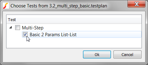
- Click Ok.Result: DVM creates the multi-step configuration file from the control symbol-defined parameters, and outputs the following curves before opening the report.
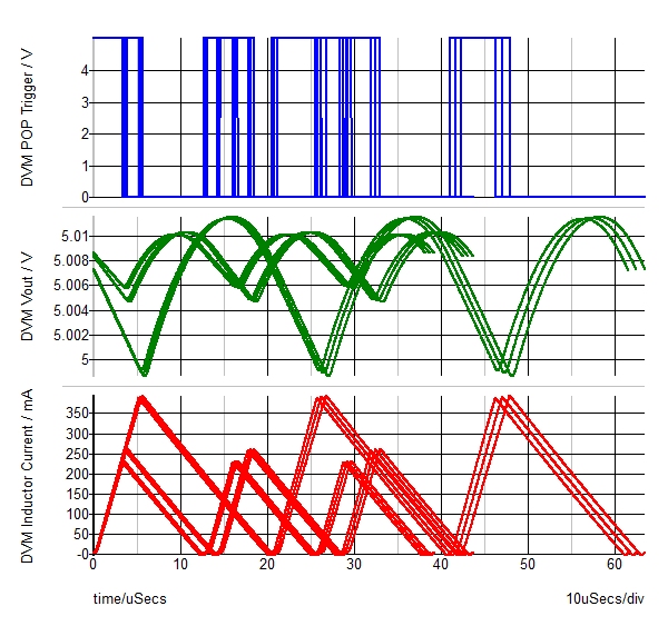
The real power of DVM lies in the HTML-formatted report generated after each test
suite runs. DVM automatically makes each probe measurement on each simulation
step, and outputs the data to the report. In the report, the stepped parameter
values and the measurements are shown in a single table: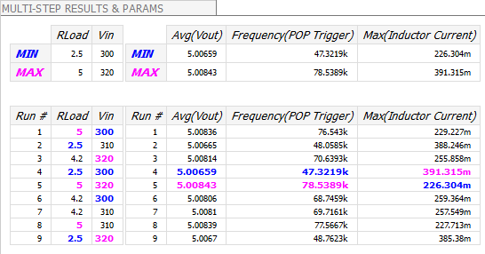
Conclusions and Key Points to Remember
- The SIMPLIS Multi-Step analysis allows you to step a parameter through a list, or to sweep a parameter with linear or decade steps to evaluate the circuit performance.
- Multiple parameters can be stepped by editing the multi-step configuration file in a text editor.
- Multi-Core capability greatly reduces the time required to execute Multi-Step simulations.
- DVM allows you to quickly and easily step parameter values and collect probe measurements from each simulation step.