User Manual: Multi-step and Monte Carlo Analyses

Overview

The SIMetrix environment provides a facility to run automatic multiple SIMPLIS analyses. Two modes are available namely parameter step and Monte Carlo.

In parameter step mode, the run is repeated while setting a parameter value at each step. The parameter may be used within any expression to describe a device or model value.

In Monte Carlo mode runs are simply repeated the specified number of times with random distribution functions enabled. Distribution functions return unity in normal analysis modes but in Monte Carlo mode they return a random number according to a specified tolerance and distribution. Any model or device parameter may be defined in terms of such functions allowing an analysis of manufacturing yields to be performed.

Comparison Between SIMetrix and SIMPLIS

The multi-step analysis modes offered in SIMetrix simulation mode achieve the same end result as the SIMPLIS multi-step modes but their method of implementation is quite different.

SIMetrix multi-step analyses are implemented within the simulator while the SIMPLIS multi-step analyses are implemented by the front end using the scripting language. The different approaches trade off speed with flexibility. The approach used for SIMPLIS is more flexible while that used for SIMetrix is faster.

Setting up a SIMPLIS Multi-step Parameter Analysis

An Example

We will begin with an example and will use one of the supplied example schematics. First open the schematic Examples/SIMPLIS/Manual_Examples/Example1/example1.sxsch. We will set up the system to repeat the analysis three times while varying R3. Proceed as follows:

First we must define R3's value in terms of an expression relating to a parameter. To do this, select R3 then press shift-F7. Enter the following:
```
{r3_value}
```
r3_value is an arbitrary parameter name. You could also use 'R3'.
Select menu Simulator | Select Multi-step...
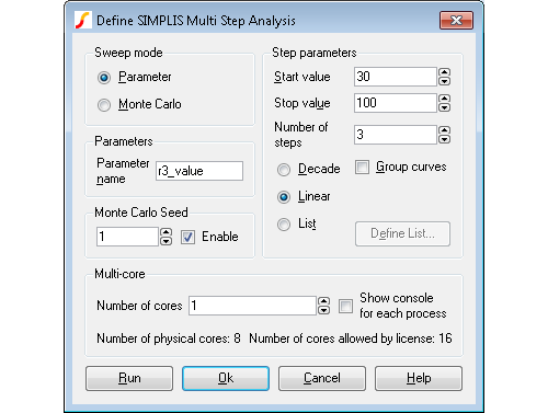
Enter 'r3_value' for Parameter Name and set Start value to 20, Stop value to 100 and Number of steps to 3. This should be what you see:
Press Run.

The analysis will be repeated three times for values of r3_value of 20, 60 and 100. The resistor value R3 is defined in terms of r3_value so in effect we are stepping R3 through that range.

In most cases you will probably want to step just one part in a similar manner as described above. But you can also use the parameter value to define any number of part or model values.

If you now run a normal single analysis, you will find that SIMPLIS reports an error as it is unable to resolve the value for R3. This can be overcome by specifying the value using a .VAR control. Add this line:

.VAR r3_value=100

to the F11 window. This line defines the value of R3 when a normal single step analysis is run.

Options

The above example illustrates a linear multi-step parameter run. You can also define a decade (logarithmic) run and also a list based run that selects parameter values from a list. To set up a list run, select the List radio button, then press Define List... Enter the values for the list using the dialog box.

The Group Curves check box controls how graphs are displayed. If unchecked, curves for each run will have their own legend and curve colour. If checked, curves will all have the same colour and share a single legend.

Setting Up a SIMPLIS Monte Carlo Analysis

An Example

To set up a Monte Carlo analysis. you must first define part tolerances. This is done by defining each value as an expression using one of the functions Gauss(), Unif or WC(). Here is another example. Open the same example circuit as above then make the following changes:

Select R3, press shift-F7 then enter the value
```
{100*GAUSS(0.05)}
```
Select C2, press shift-F7 then enter the value
```
{100u*GAUSS(0.2)}
```
Delete the fixed probes on the V1 input and on R1. (This is just to prevent too many unnecessary curves being plotted)

The above will give R3 a 5% tolerance and C2 a 20% tolerance with a 3 Sigma Gaussian distribution. Now set up the Monte Carlo run:

Select menu Simulator > Setup Multi-step...
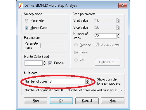
In Sweep mode select Monte Carlo
Enter the desired number of steps in Number of steps. To demonstrate the concepts, 10 will be sufficient, but usually a Monte Carlo run would be a minimum of around 30 steps
Press Run

You should see a series of curves build up as the run progresses.

Multi-core Multi-step SIMPLIS Analyses

If your system and your license permit, you can specify multiple processor cores to be employed for multi-step analyses. This can substantially speed up the run. For example, suppose you have a 4 core system and wish to run a 100 step Monte Carlo analysis. The 100 steps may be split across the 4 cores each doing 25 steps each. In most cases this improve the run time by at least a factor of 3.

In this mode of operation, multiple SIMPLIS processes run independently with each one creating its own data file.

To setup a Multi-core Multi-step SIMPLIS Analysis

Setup the multi-step analysis as normal. In the Define SIMPLIS Multi Step Analysis dialog box set the Number of cores to the desired value as shown below. Note that the maximum value you can set is determined by your license and system. For allowed number of cores for each product type, see Simulation and Multi-core Processors.

Running a SIMPLIS multi-core multi-step analysis

Start the run in the usual way for a multi-step run. You will see the usual SIMPLIS status box but with the difference that there will be multiple tabs, one for each process running as shown below:

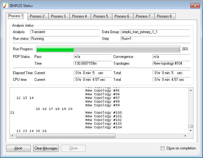
You can watch the progress of each process using the tabs at the top of the status box.

Using Fixed Probes with SIMPLIS Multi-core Multi-step Analyses

Fixed probes usually update the waveform viewer incrementally. That is, the display is updated while the simulation proceeds. This does not happen for multi-core multi-step runs. Instead, the graphs will be updated when the run is complete.

Tolerances and Distribution Functions

Distribution Functions

Tolerances are defined using distribution functions. For SIMPLIS Monte Carlo there are just three functions available. These are defined below.

Function Name	Description
GAUSS(tol)	Returns a random with a mean of 1.0 and a standard deviation of tol/3. Random values have a Gaussian or Normal distribution.
UNIF(tol)	Returns a random value in the range 1.0 +/- tol with a uniform distribution
WC(tol)	Returns either 1.0-tol or 1.0+tol chosen at random.

The 'L' and 'E' suffix functions available in SIMetrix Monte Carlo analysis are not available for SIMPLIS operation.

Lot and Device Tolerances

No special provision has been made to implement so called 'Lot' tolerances which model tolerances that track. However, it is nevertheless possible to implement Lot tolerances by defining a parameter as a random variable. Suppose for example that you have a resistor network consisting of 4 resistors of 1k with an absolute tolerance of 2% but the resistors match to within 0.2%. The absolute tolerance is the 'lot' tolerance. This is how it can be implemented:

Assign a random variable using the .VAR preprocessor control. (You cannot use .PARAM in SIMPLIS simulations). E.g.:
```
.VAR rv1 = {UNIF(0.02)}
```
Give each resistor in the network a value of:
```
{1K * rv1 * UNIF(0.002)}
```

rv1 will be updated on each Monte Carlo step but will always have the same value in each place where it is used.

Monte Carlo Log File

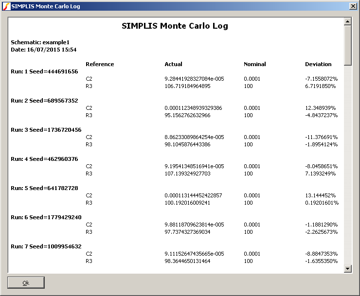
When a Monte Carlo analysis is run a log file is created which details which device values were changed and what they were changed to. Two versions of the log file are created; one is plain text and is called simplis_mclog.log and the other is in HTML format and called simplis_mclog.html.

To view the HTML log file, select menu Monte Carlo > View Log File

An example is shown below:

Monte Carlo Seed Values

Introduction

The random values used in Monte Carlo analysis are generated using a pseudo-random number generator. This generates a sequence of numbers that appear to be random and have the statistical properties of random numbers. However, the sequence used is in fact repeatable by setting a defined seed value. The sequence generated will always be the same as long as the same starting seed value is used.

This makes it possible to repeat a specific Monte Carlo step as long as the seed value is known. SIMetrix/SIMPLIS explicitly sets a random seed value at the start of each Monte Carlo run and records this in a file. A facility exists to explicitly set the seed value instead of using a random seed and this makes it possible to repeat a specific step. This is useful in cases where one or more Monte Carlo steps show unexplained behaviour and further investigation is needed.

This is also useful if you wish to find the values of the parts used for a particular Monte Carlo step.

Finding the Seed Value

To find the seed value of a particular step, follow this procedure:

Run normal Monte Carlo without seed definition if you have not done so already.
Find the run number of the result whose seed you require (so that you can repeat that step). You can find the run number from a plotted waveform from the Monte Carlo run. Plot a result as normal then switch on cursors. Place the cursor on the curve of interest then select menu Cursors > Show Curve Info. The run number will be displayed in the command shell. For more information about graph cursors see Graph Cursors.
Select menu Monte Carlo > View Log File to show the log file. The seed value is shown against the run number. See Monte Carlo Log File

Using the Seed Value

You can use the seed value to repeat the run associated with it. Follow this procedure:

Select menu Simulator > Setup Multi-step. In the Monte Carlo Seed group check the Enable box and enter the seed value obtained from step 3 in the above section. Set the Number of steps to 1.
Run the simulation as normal.

Finding Part Values Used

The part values used for a particular step can be found by studying the .deck file that is created for every SIMPLIS run. To do this, follow the procedure for finding and using the seed value as described above. Then after the single run is complete locate the file with the .deck extension. This will be located in the SIMPLIS_DATA folder and will have a name the same as the top level schematic but with the extension .deck. So if your schematic is called DC-DC-Converter.sxsch, the deck file will be called DC-DC-Converter.deck and will be located in the SIMPLIS_DATA folder.

The .deck file is an ASCII file that list the parts in the design with their connections and values. Its format is similar to a SPICE netlist. The picture below illustrates the process of matching a part in the schematic to an entry in the .deck file:

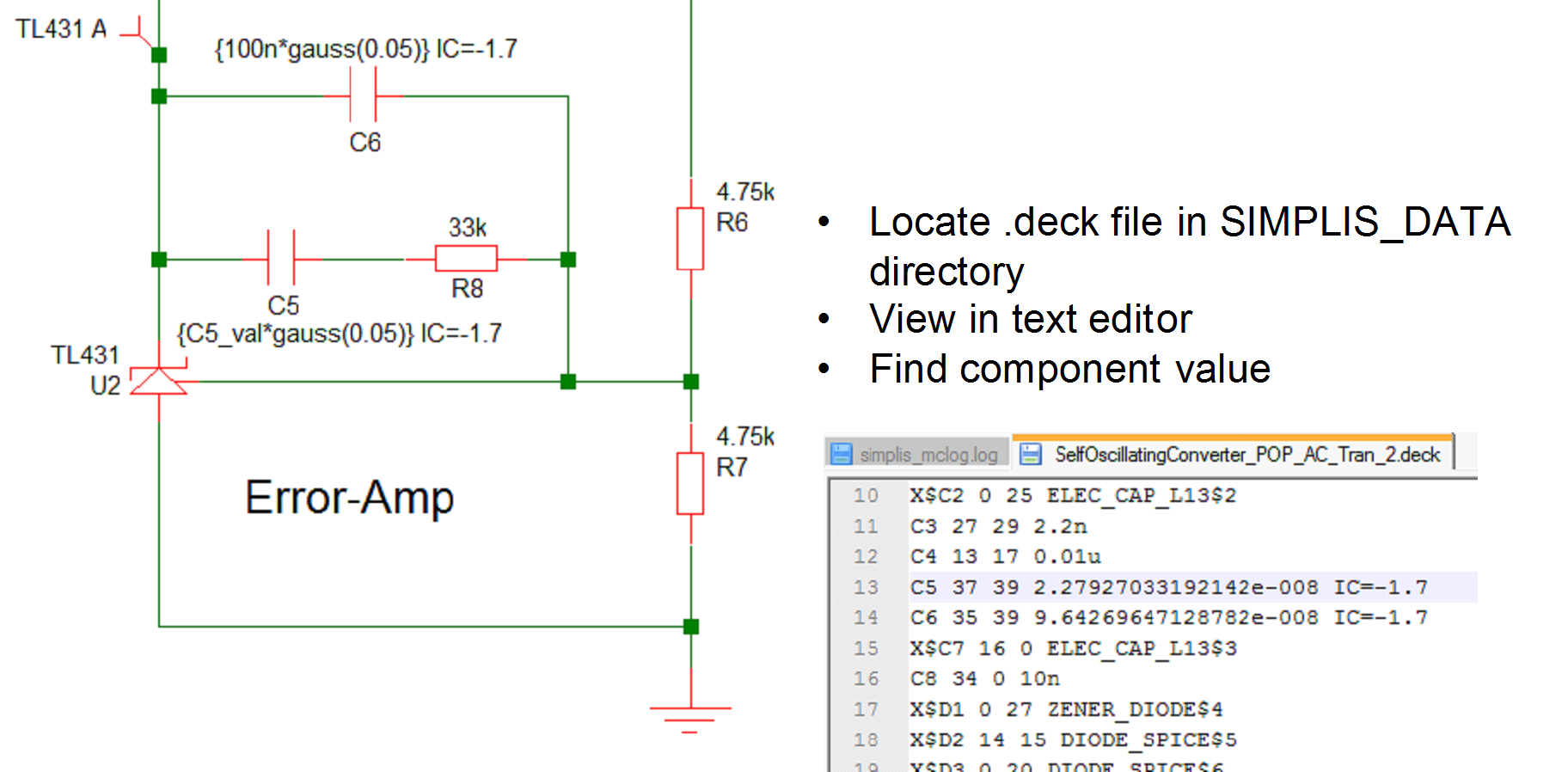
In the above diagram, note the line for C5 shows a value of 2.2797033192142e-008 in the .deck file

Performance Analysis and Histograms

Once a SIMPLIS multi-step or Monte Carlo analysis is complete, the data can be analysed in exactly the same way as for SIMetrix multi-step analyses. This includes the performance analysis and histogram features. For more information, see Performance Analysis and Histograms.