IIR Function
Performs Infinite Impulse Response digital filtering on supplied vector. This function performs the operation:
\[ y_n = x_n c_0 + y_{n-1}c_1 + y_{n-2}c_2 \dots \]
| ???MATH???x???MATH??? | is the input vector (argument 1) |
| ???MATH???c???MATH??? | is the coefficient vector (argument 2) |
| ???MATH???y???MATH??? | is the result (returned value) |
The operation of this function (and also the function FIR ) is simple but its application can be the subject of several volumes! In principle an almost unlimited range of IIR filtering operations may be performed using this function. Any text on Digital Signal Processing will provide further details.
User's should note that using this function applied to raw transient analysis data will not produce meaningful results as the values are unevenly spaced. If you apply this function to simulation data, you must either specify that the simulator outputs at fixed intervals (select the Output at .PRINT step option in the dialog box) or you must interpolate the results using the function Interp .
Arguments
| Number | Type | Compulsory | Default | Description |
| 1 | real array | Yes | Vector to be filtered | |
| 2 | real array | Yes | Coefficients | |
| 3 | real array | No | zero | Initial conditions |
Returns
Return type: real array
Example
The following graph shows the result of applying a simple first order IIR filter to a
step:
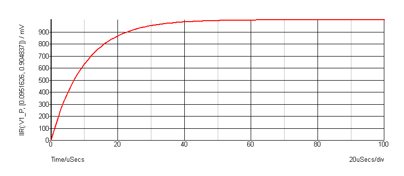 The coefficients used give a time constant of 10 * the sample interval. In the above the
sample interval was ???MATH???1\mu???MATH???Sec so giving a ???MATH???10\mu???MATH???Sec time constant. As can be seen a first
order IIR filter has exactly the same response as an single pole RC network. A general
first order function is:
\[
y_n = x_nc_0 + y_{n-1}c_1
\]
where ???MATH???c_0 = 1 - \exp\left(\frac{-T}{\tau}\right)???MATH???
and ???MATH???c_1 = \exp\left(\frac{-T}{\tau}\right)???MATH???
and ???MATH???\tau = \text{time constant}???MATH???
and ???MATH???T = \text{sample interval}???MATH???
The above example is simple but it is possible to construct much more complex filters
using this function. While it is also possible to place analog representations on the
circuit being simulated, use of the IIR function permits viewing of filtered waveforms
after a simulation run has completed. This is especially useful if the run took a long
time to complete.
The coefficients used give a time constant of 10 * the sample interval. In the above the
sample interval was ???MATH???1\mu???MATH???Sec so giving a ???MATH???10\mu???MATH???Sec time constant. As can be seen a first
order IIR filter has exactly the same response as an single pole RC network. A general
first order function is:
\[
y_n = x_nc_0 + y_{n-1}c_1
\]
where ???MATH???c_0 = 1 - \exp\left(\frac{-T}{\tau}\right)???MATH???
and ???MATH???c_1 = \exp\left(\frac{-T}{\tau}\right)???MATH???
and ???MATH???\tau = \text{time constant}???MATH???
and ???MATH???T = \text{sample interval}???MATH???
The above example is simple but it is possible to construct much more complex filters
using this function. While it is also possible to place analog representations on the
circuit being simulated, use of the IIR function permits viewing of filtered waveforms
after a simulation run has completed. This is especially useful if the run took a long
time to complete.
| ▲Function Summary▲ | ||
| ◄ IffV | im ▶ | |