6.1.2 Constant Current Subcircuit
To download the examples for Module 6, click Module_6_Examples.zip
In this topic:
What You Will Learn
- How to create a constant current subcircuit load using a Piecewise Linear (PWL) Resistor.
- How to calculate a parameter value using if/else branching constructs.
- PWL resistors require the first and last segments to have positive resistance.
Model Requirements
The constant current load should:
- Model a constant current for voltages above a minimum saturation voltage.
- Allow users to optionally add a parasitic shunt resistance to the load.
- Limit the valid parameter values, including the calculated parameter values, to a range of values.
- Include a tabbed parameter editing dialog.
- Be self-contained in a schematic component file.
Model Design Procedure
The design procedure for this model is broken into four logical parts.
- Part 1: Add PWL Resistor and Rename Constant Resistance Load File
- Part 2: Parametrize the PWL Resistor
- Part 3: Define Calculated Parameters
- Part 4: Check Passed Parameter Values With .ERROR
Part #1: Add PWL Resistor and Rename Constant Resistance Load File
You will start the model by opening the constant_resistance_load.sxcmp file you created in the 6.1.1 Constant Resistance Subcircuit topic. You will then add a voltage-controlled PWL resistor symbol and save this schematic component to a new file.
- Open the constant_resistance_load.sxcmp schematic component created during the 6.1.1 Constant Resistance Subcircuit. If you haven't created this file, open the "answer" file: 6.1.1_constant_resistance_load_answer.sxcmp.
- Select R1, and press the Delete key to delete the resistor symbol.
- On the Schematic Editor window, click on the toolbar search icon:
 .Result: The search dialog opens:
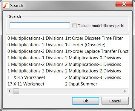
- Enter pwl in the Search box. Result: The list of SIMPLIS compatible devices containing the text string pwl (case-insensitive) is displayed below the Search field:
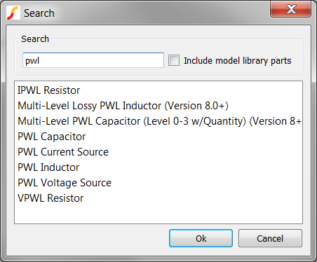
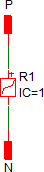
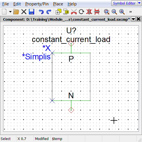
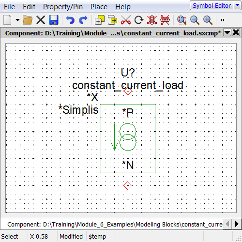
- Select the last item, the VPWL Resistor, and place it on the schematic
where the Z-shaped resistor was located. The schematic should appear as
follows:
- From the Schematic Editor menu, select
- Enter constant_current_load.sxcmp in the File name field and click Save to save the schematic component.
A point to remember: When you save a schematic component file using the Save Schematic As... menu option, only the schematic portion is saved and the symbol is discarded. In this case, you do not want to retain the graphical portions of the symbol, so this makes sense. To rename and save a schematic component file including the symbol, use the menu option, and check the Complete component including symbol checkbox.
Part #2: Parametrize the PWL Resistor
In this part, you will define the PWL resistor points using parameter values. The constant current load requires four parameters which the user will enter on the parameter editing dialog. These parameter names and the default values are shown in the table below:
| Parameter Description | Parameter Name | Default Parameter Value |
| The constant load current in amps | DC_CURRENT | 1 |
| The load saturation voltage in volts | SAT_VOLTAGE | 0.2 |
| The parallel, or shunt resistance in ohms | RSHUNT | 10Meg |
| A boolean flag to use the parallel resistance in the circuit | USE_RSHUNT | 1 |
There are several ways to add these parameters to the actual PWL resistor. For this model you will define parameters calculated in the F11 window in addition to the parameters passed into the subcircuit through the symbol. In addition to the four parameters passed into the subcircuit through the symbol, the following four calculated parameters will be used:
| Parameter Description | Parameter Name |
| Third voltage point | VOLTAGE_3 |
| Third current point | CURRENT_3 |
| Fourth voltage point | VOLTAGE_4 |
| Fourth current point | CURRENT_4 |
The resulting V-I curve for the load with the parameters annotated is shown below. Each voltage-current pair is annotated in (x,y) format. How the four additional parameters are calculated will be covered in Part 3: Define Calculated Parameters.
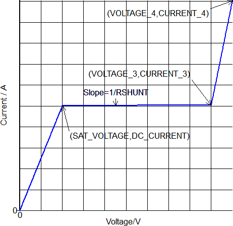
Notice the last segment in the resistor has a positive slope. SIMPLIS requires all PWL resistors to have positive slope for both the first and last PWL segment, and this model allows users to define the load as a ideal current source. If you did not add this third segment, the model would produce an error message because the slope of the last segment would be zero. This segment is placed at a voltage which is well beyond the operating voltage range of the load, preventing the final segment from effecting the normal operation of the load.
To parameterize the PWL resistor,
- Double click on the PWL resistor R1. Result: The Define VPWL Resistor: R1 dialog opens:
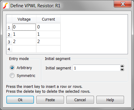
- Stretch the Voltage and Current columns to approximately twice the
default width.
- Position the mouse between the Voltage and Current Columns on
the title bar row. Result: The mouse cursor changes to two vertical bars, indicating the columns are ready to be re-sized.
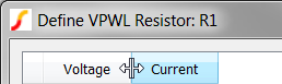
- Press and hold the left mouse button and drag the column to re-size.
- Repeat for the Current column by moving the mouse cursor to the right of the Current column, and repeating step B.
- Position the mouse between the Voltage and Current Columns on
the title bar row.
- Starting at the second data point, enter {SAT_VOLTAGE} in the Voltage
column and {DC_CURRENT} in the Current column. Double-click the left mouse
button to change table cells, by default this selects all text in the table cell.
Result: The dialog at this point appears as follows:
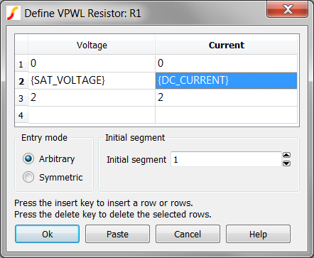 CAUTION:Spelling errors here will have disastrous consequences later on. Whenever you enter text by hand, double check the spelling. A good way to avoid spelling errors is to copy and paste the text from this document.
 - Repeat Step #3 entering {VOLTAGE_3} and {CURRENT_3} in the third
row and {VOLTAGE_4} and {CURRENT_4} in the fourth row. Result: The final dialog is configured as follows:
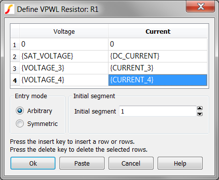
- Click Ok to save the changes.
At this point, the PWL resistor uses six parameters - two are passed in from the symbol, and the other four are calculated from the passed-in parameters. In the next part, you will define the four calculated parameters in the F11 window of the constant_current_load.sxcmp schematic component.
Part #3: Define Calculated Parameters
The first two data points which define the PWL resistor are either constants or passed into the subcircuit from the symbol. The third and fourth points are either constant, or calculated from the parameters passed into the subcircuit. In this part, you will define these parameters in the F11 window of the schematic component.
Using the F11 window of the schematic component to define local parameters is good modeling technique. These local parameters can be constants, or calculated from the parameters passed into the subcircuit. Once a parameter is defined in the F11 window, it can be used in other calculations which occur later in the same F11 window. You can think of the parameters which are passed into the subcircuit through the symbol as being at the very top of the F11 window. These parameters can be used anywhere in the F11 window to define new parameters.
- Press F11 to open the command (F11) window.
- Select all text in the F11 window Ctrl+A and delete it.
- The third voltage point is set by parameter VOLTAGE_3 and should be placed
well above the normal operating voltage for the load. A voltage of 10,000V would
be comfortably above the maximum operating voltage for the load for most purposes.
This is an example of a constant parameter defined in the F11 window. Enter the
following text in the F11 window of the schematic:
.VAR VOLTAGE_3 = 10000
- Next, the CURRENT_3 parameter needs to be calculated. The value of
CURRENT_3 depends on the USE_RSHUNT parameter. If the
USE_RSHUNT parameter is a logical true (non-zero), the CURRENT_3
parameter includes the RSHUNT parameter. If the USE_RSHUNT parameter
value is zero, the load models a pure current source with infinite output
impedance over the operating voltage range of VSAT_VOLTAGE to
VOLTAGE_3. The following .IF/.ELSE/.ENDIF construct can be used to
define the CURRENT_3 parameter value. Enter the following text in the F11
window of the schematic:
.IF { USE_RSHUNT } .VAR CURRENT_3 = { DC_CURRENT + ( VOLTAGE_3 - SAT_VOLTAGE ) / RSHUNT } .ELSE .VAR CURRENT_3 = { DC_CURRENT } .ENDIF - Finally, the values of last voltage and current pair are defined to add a 1Ω
positive slope. These parameters are a function of the VOLTAGE_3 and
CURRENT_3 parameters. Enter the following text in the F11 window of the
schematic:
.VAR VOLTAGE_4 = { VOLTAGE_3 + 1 }
.VAR CURRENT_4 = { CURRENT_3 + 1 }
Result: The F11 window should appear as follows: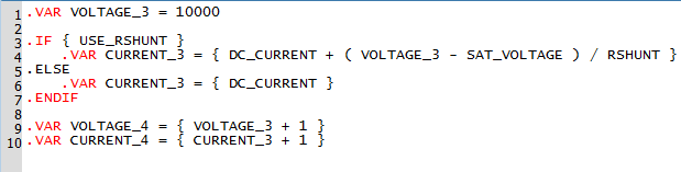
Note that the parameters are dependent on previous parameters in the same F11 window. The first parameter defined is VOLTAGE_3. Depending on the value of the USE_RSHUNT parameter, the value of CURRENT_3 can depend on the value of VOLTAGE_3. The values of both CURRENT_4 and VOLTAGE_4 are then dependent on the values of CURRENT_3 and CURRENT_4. The ability to define parameters which are dependent on previous parameters is one of the key benefits to using the F11 window to define calculated parameters.
At this point, all PWL resistor points are defined, but no error checking has been added. In the next step, Part 4: Check Passed Parameter Values With .ERROR, you will add error checking for the parameter values.
Part #4: Check Passed Parameter Values With .ERROR
In this part you will use the .IF/.ENDIF and .ERROR constructs to check if the parameter values are within the ranges allowed by the model.
- The first error message is similar to the one you used in 6.1.1 - Part 3. This tests that the DC_CURRENT parameter is
greater than zero. Copy the following three lines of text and paste into the F11
window.
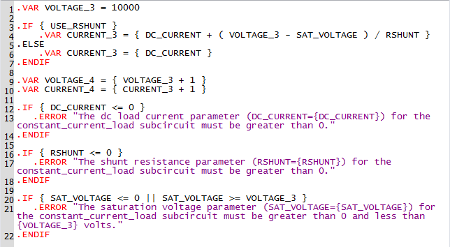
.IF { DC_CURRENT <= 0 } .ERROR "The dc load current parameter (DC_CURRENT={DC_CURRENT}) for the constant_current_load subcircuit must be greater than 0." .ENDIF - Next, the shunt resistance parameter RSHUNT is checked to ensure the
parameter value is greater than zero. Copy the following three lines of text and
paste into the F11 window.
.IF { RSHUNT <= 0 } .ERROR "The shunt resistance parameter (RSHUNT={RSHUNT}) for the constant_current_load subcircuit must be greater than 0." .ENDIF - Finally, the saturation voltage parameter SAT_VOLTAGE is checked to see if
it is greater than zero volts and less than 10k volts. This .IF statement uses the
logical OR operator - two pipe characters "||", to test if the parameter is either
less than or equal to 0V or greater than or equal to 10k volts. Copy the following
three lines of text and paste into the F11 window.
.IF { SAT_VOLTAGE <= 0 || SAT_VOLTAGE >= VOLTAGE_3 }
   .ERROR "The saturation voltage parameter (SAT_VOLTAGE={SAT_VOLTAGE}) for the constant_current_load subcircuit must be greater than 0 and less than {VOLTAGE_3} volts."
.ENDIF
After adding these three error messages, the F11 window should appear as follows:
Symbol Design Procedure
As in section 6.1.1, Symbol Design Procedure, the symbol design procedure is broken into three parts:
- Part A: Edit the Auto-Created Symbol
- Part B: Copy Graphics From Current Source Symbol
- Part C: Add Parameters and Dialog Properties
Part A: Edit the Auto-Created Symbol
To get started,you will use the built-in symbol auto-creation process to create a symbol. The auto-created symbol has all the electrically significant properties which netlist a subcircuit instantiation for a SIMPLIS simulation. You will then modify the symbol, enlarging it so the graphical elements which represent a current source will fit inside the symbol's box.
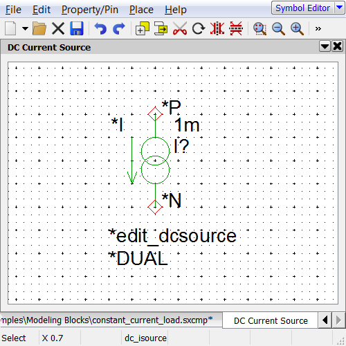
- Press S to auto-create a symbol.Result: The auto-created symbol opens in the symbol editor.
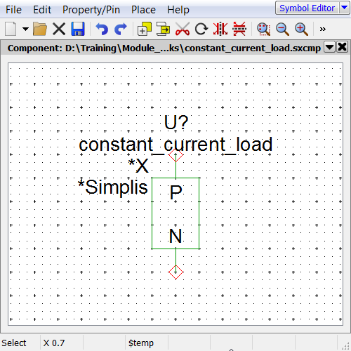
- Using the mouse, drag a selection box around the upper portion of the symbol,
including the P pin and the horizontal line.
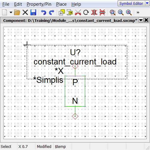 Result: The selected portions of the symbol should appear exactly as below:
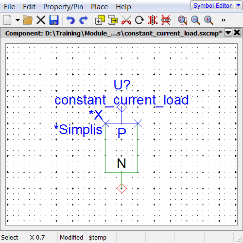
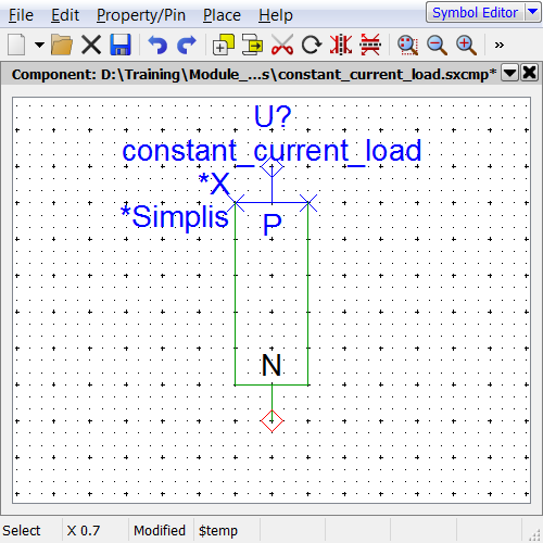
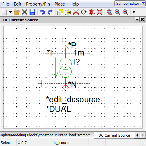
- Move the mouse over any selected item, press and hold down the left mouse button,
and drag the selected items up 2 grid squares.Result: The symbol should now look like the following:
- Using the mouse, drag a selection box around the vertical line on the right side
of the symbol:
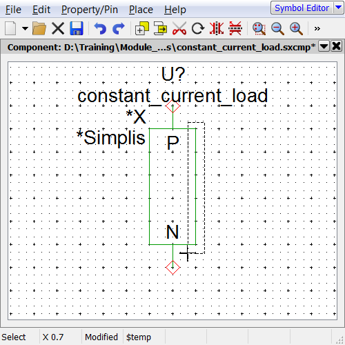 Result: The selected portions of the symbol should appear exactly as below:
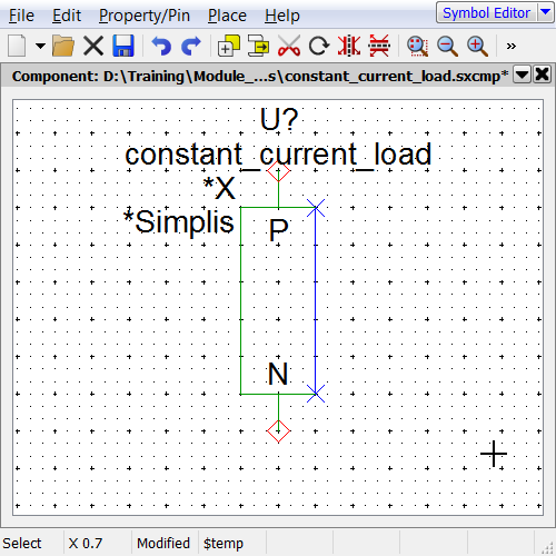
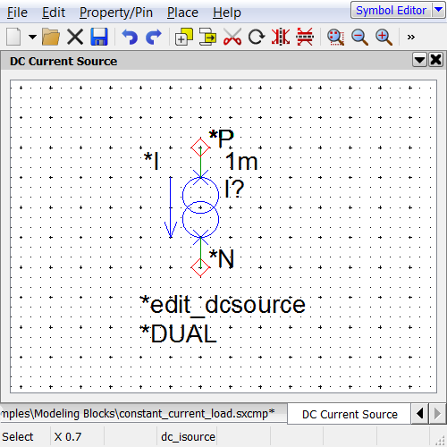
- Drag the selected line to the right one grid square.
- Repeat steps 4 and 5 for the left side vertical line.Result: The symbol should appear as follows:
- Finally, the positive and negative pin names are not needed, so you will hide
them.
- Click on the N text representing the pin name.
- Press F7 to open the Edit Pin dialog.Result: The Edit Pin dialog opens
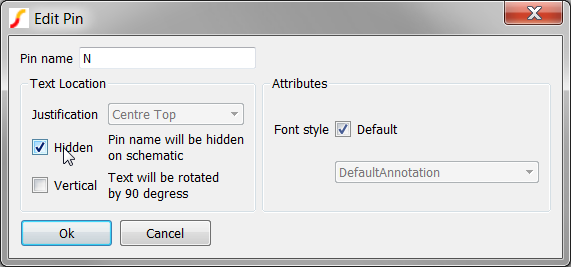
- Check the Hidden checkbox.
- Click Ok to save your changes.
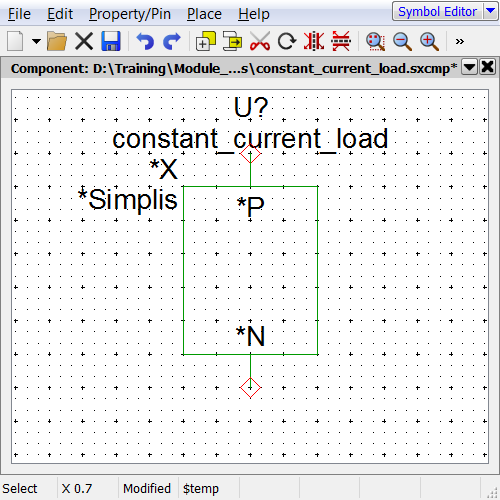
- Repeat step 7 for the P pin.Result: The final symbol will appear as follows:
At this point, the subcircuit load has a complete schematic and a pretty basic symbol. Since the load is essentially a current source, you will add a graphical current source symbol to the load. The simplest way to do this is to open the library symbol for the current source, and copy the graphical elements of the current source symbol to your symbol.
Part B: Copy Graphics From Current Source Symbol
- From the symbol editor menu, select .Result: The Select Symbol dialog opens
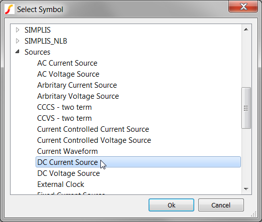
- Click on the Sources category, then on the DC Current Source entry.
- Click Ok.Result: The symbol opens in the symbol editor
- You now have both your schematic component symbol and the built-in DC Current Source symbol open in the symbol editor
- Use the mouse to drag a selection box around the graphical elements of the DC
Current Source symbol. The selection box should appear as follows:
 Result: The selected items should appear as follows:
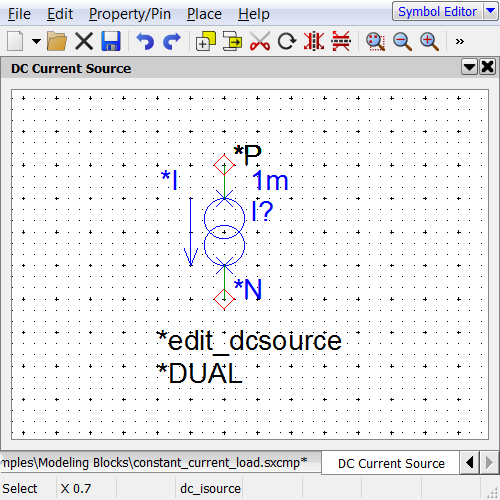
- This selection box will select the graphical elements of the current source
symbol as well as the other symbol properties and the N pin. Next you will
unselect the symbol properties, leaving the two circles and the arrow selected.
- To unselect any graphical element or symbol property, press and hold the Ctrl key while left clicking on that element.
- Repeat this process for each symbol property and the N pin.Result: The correctly selected lines and circles are as follows:
- Copy the selected lines and circles to the clipboard using Ctrl+C.
- Select the symbol editor tab with your schematic component symbol.
- Paste the current source symbol elements in the center of your symbol.Result: Your symbol should look like the following:

- Add lines to connect the circles to the pins. The final symbol should appear as
follows:
- Finally, change the default reference designator to LOAD?.
- Click on the U? symbol property value.
- Press F7 to edit the property
- Change the value to LOAD?
- Click Ok to save your reference property changes.
- Press Ctrl+S to save your symbol to the schematic component file.
- Close the DC Current Source symbol without saving it.
You now have a symbol which will call the subcircuit based current source load model. The functionality of the underlying subcircuit is implied by the current source symbol, and the box around the current source suggests to the user that this is not a normal current source. At this point the symbol doesn't pass parameters to the underlying subcircuit, nor does the symbol have a parameter editing dialog. In the next part, Part C: Add Parameters and Dialog Properties, you will use a spreadsheet to add the required symbol properties.
Part C: Add Parameters and Dialog Properties
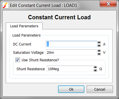
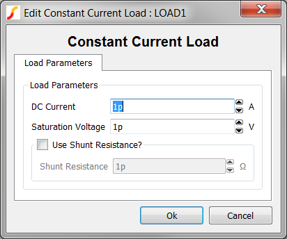
Included in the Module_6_Examples.zip file is a pre-prepared dialog definition spreadsheet similar to the one used in the previous module. Like the spreadsheet used in 6.1.1 Part #2: Add RESISTANCE Parameter and Dialog Properties, this spreadsheet contains all the script commands required to add the properties to the symbol. The extracted file is located at: C:\Training\Module_6_Examples\6.1.2_constant_current_load_dialog_definition_worksheet.xlsx. The dialog definition creates the following dialog for the constant current load:
To add the symbol properties:
- Open the 6.1.2_constant_current_load_dialog_definition_worksheet.xlsx excel spreadsheet.
- Copy the 11 cells: B37-B47 to the windows clipboard.
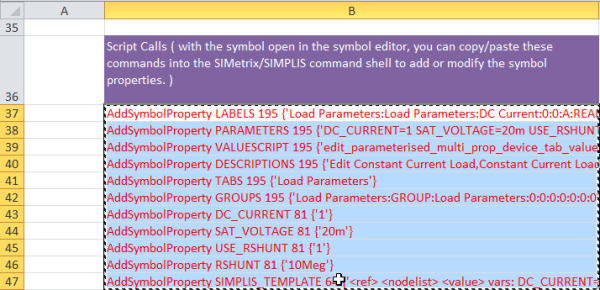
- Navigate to the SIMetrix/SIMPLIS command shell window.
- Click the mouse in the command line entry located at the top of the command
shell:
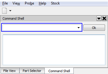
- Press Ctrl+V to paste the commands in the command line.Result: the last command is partially visible in the command line.
- Press Enter or click the Ok Button on the command line.Result: The commands are executed in SIMetrix/SIMPLIS. Each AddSymbolProperty command adds a single symbol property to the symbol. As in previous exercises, the dialog definition properties are protected. All properties are hidden from view when the symbol is placed on the parent schematic.

- Press Ctrl+S to save your symbol to the schematic component file. Click Ok on the Save symbol dialog.
Test the Model
Now that the model and associated symbol are completed, its time to start testing. A testbench schematic for the constant current load is located in the Module_6_Examples directory. After you place the load, this test schematic is ready to simulate. You will then run a few experiments on the model to verify it works as expected.
To start testing the model:
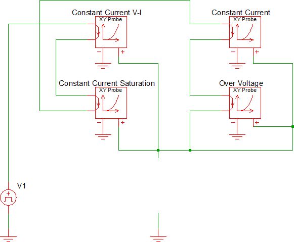
- Open the 6.2_test_constant_current.sxsch schematic.Result: The testbench schematic opens, this schematic has been specially prepared to test the load using four XY probes and a ramped voltage source. Each X-Y probe is configured to display one of the three PWL resistor operating segments.
- From the Schematic Editor menu select
- Select the constant_current_load.sxcmp component file from the Modeling Blocks directory.
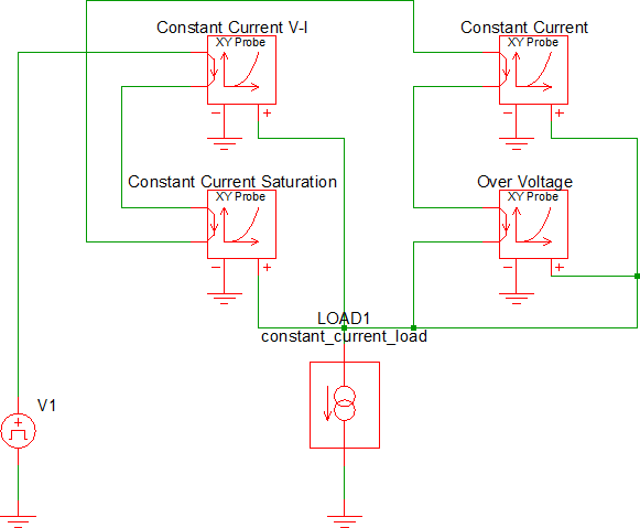
- Place the load on the schematic below the 4 probes.
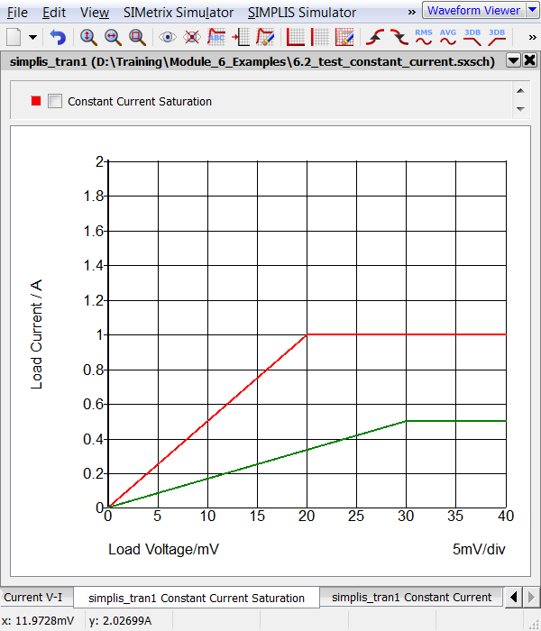
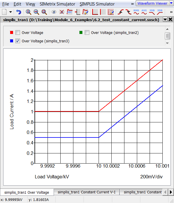
- Press F9 to run the simulation. Result: The V-I curves for the load are generated on three tabs. The last tab displays the load characteristics over the full operating range.

Each graph tab displays a different operating region for this load. The individual X-Y probes have been configured to set the graph X-values to a range appropriate to the default load parameters. For example, the default saturation voltage is 20mV. The saturation graph is displayed over a X range of 0 to 40mV. The vertical axis is auto scaled to fit the data. In this case, the actual curve extends to a load voltage of 10,001V, at which the current is approximately 2A. For this reason, the graph is auto scaled to a maximum Y-value of 2A.
Experiment #1: Test Dialog and Change Parameter Values
Whenever you pass parameters to subcircuits, it is important to test that the parameters are being passed properly and the simulation results reflect the actual parameter value. In this experiment, you will change the load parameters and verify the value changes in the simulation.
- Navigate to the Schematic Editor window.
- Double click on the subcircuit load symbol to edit the resistance parameter.
Result: The parameter editing dialog opens.
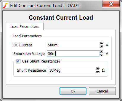
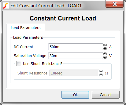
- Change the DC Current value to 500m, and change the Saturation Voltage parameter to 30m and click Ok to accept the dialog. The dialog should appear as follows:
- Press F9 to run the simulation.
Result: The green V-I curve for the load is generated with the new parameters.
Experiment #2: Test USE_RSHUNT Logic
Next you will check the USE_RSHUNT logic is working properly.
- Double click on the LOAD1 symbol to edit the parameters
- Uncheck the Use Shunt Resistance? check box. Result: The Shunt Resistance parameter control is disabled (grayed-out), suggesting to the user that the Shunt Resistor will not be used in the model.
- Click Ok to save your changes.
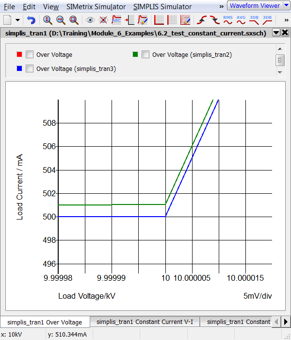
- Press F9 to run the simulation. Result: A third set of curves is overlaid on the waveform viewer:
- Select the first tab with the over voltage characteristics:
- Zoom into the point at which the blue curve changes slope.
- While pressing and holding the left mouse button, drag a box selection around the point where the blue curve changes slope. This is the transition from the constant current segment to the over voltage segment.
- Release the left mouse button. You may need to zoom multiple times to get
to a magnification which allows you to see the shunt resistance effect.
Result: The graph clearly shows the current at the 10kV point is approximately 501mA, which is the 500mA DC Current plus the shunt resistance contribution. The shunt resistance contributes 10kV/10MegΩ or 1mA to the load current at the load voltage of 10kV.
Experiment #3: Test .ERROR Message
Testing the .ERROR message is slightly more difficult because the parameter editing dialog will not allow you to enter an invalid value. Instead you will manually edit the value using the Edit Properties dialog.
- Select the LOAD1 symbol.
- Right click and select the Edit/Add Properties... menu option.
Result: The Edit Properties dialog opens:
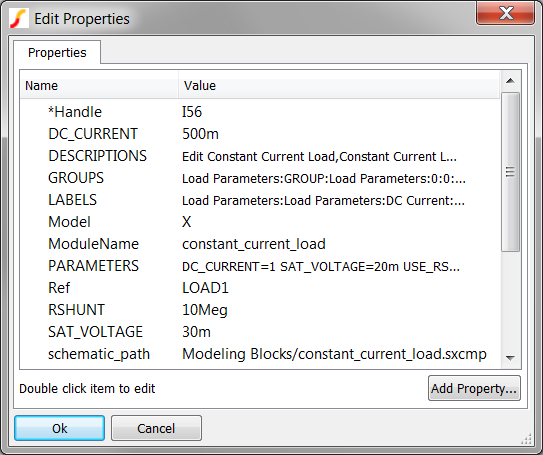
- Change the DC_CURRENT, RSHUNT, and SAT_VOLTAGE properties to 0.
- Double click on each property. On the Edit Property dialog, change each property Value to 0, and click Ok on the Edit Property dialog to accept the changes.
- Repeat for each property.
- Click Ok on the Edit Properties dialog.
- Press F9 to run the simulation.Result: All three parameters are less than the minimum limit specified in the F11 window of the constant_current_load.sxcmp schematic, and each .ERROR statement is output to the command shell:
*** ERROR *** (6.2_test_constant_current.net;55): Subckt def constant_current_load used by X$LOAD1:
The saturation voltage parameter (SAT_VOLTAGE=0) for the constant_current_load subcircuit must be greater than 0 and less than 10000 volts.
*** ERROR *** (6.2_test_constant_current.net;51): Subckt def constant_current_load used by X$LOAD1:
The shunt resistance parameter (RSHUNT=0) for the constant_current_load subcircuit must be greater than 0.
*** ERROR *** (6.2_test_constant_current.net;47): Subckt def constant_current_load used by X$LOAD1:
The dc load current parameter (DC_CURRENT=0) for the constant_current_load subcircuit must be greater than 0.
Experiment #4: Test Minimum Values Allowed by Dialog
In the previous experiment you set the load parameters to values less than the minimum allowed by the parameter editing dialog. In this short experiment you will verify the dialog prevents users from entering values less than the specified minimum value.
- Double click on the LOAD1 symbol to open the parameter editing dialog.
Result: Although the three parameters were set to 0 in the last exercise, the dialog automatically changes the values to 1p, which is the minimum allowed value for each parameter. The 1p value is defined in the Excel spreadsheet for this dialog definition.
- Press the up arrow button on the DC Current spinner control. Result: The DC Current value changes from 1p to 2p.
- Press the down arrow button twice on the DC Current spinner control.
Result: The DC Current value changes from 2p to 1p , and on the second click, the minimum value of 1p is enforced.
Conclusions and Key Points to Remember
A PWL resistor can be used to define a very flexible constant current load. This load will simulate without producing numerical errors if the terminals are left open circuited.
Key points to remember are:
- You can define parameters local to the F11 window. These parameters can be constants or be defined in terms of the parameters passed into the subcircuit.
- You can further test the value of parameters passed into the subcircuit with the .IF/.ELSE statements to define new parameters.
- You can validate parameter values are within a range with the .ERROR statement. Any parameter can be checked, including calculated parameters.
- When parametrizing PWL resistors, make certain the first and last segments have a positive slope.